⇐ Previous topic|Next topic ⇒
Table of Contents
Statistics of dispersion
Summary
A statistic of dispersion tells you how spread out a set of measurements is. Standard deviation is the most common, but there are others.
Introduction
Summarizing data from a measurement variable requires a number that represents the "middle" of a set of numbers (known as a "statistic of central tendency" or "statistic of location"), along with a measure of the "spread" of the numbers (known as a "statistic of dispersion"). You use a statistic of dispersion to give a single number that describes how compact or spread out a set of observations is. Although statistics of dispersion are usually not very interesting by themselves, they form the basis of most statistical tests used on measurement variables.
Range: This is simply the difference between the largest and smallest observations. This is the statistic of dispersion that people use in everyday conversation; if you were telling your Uncle Cletus about your research on the giant deep-sea isopod Bathynomus giganteus, you wouldn't blather about means and standard deviations, you'd say they ranged from 4.4 to 36.5 cm long (Biornes-Fourzán and Lozano-Alvarez 1991). Then you'd explain that isopods are roly-polies, and 36.5 cm is about 14 American inches, and Uncle Cletus would finally be impressed, because a roly-poly that's over a foot long is pretty impressive.
Range is not very informative for statistical purposes. The range depends only on the largest and smallest values, so that two sets of data with very different distributions could have the same range, or two samples from the same population could have very different ranges, purely by chance. In addition, the range increases as the sample size increases; the more observations you make, the greater the chance that you'll sample a very large or very small value.
There is no range function in spreadsheets; you can calculate the range by using =MAX(Ys)−MIN(Ys), where Ys represents a set of cells.
Sum of squares: This is not really a statistic of dispersion by itself, but I mention it here because it forms the basis of the variance and standard deviation. Subtract the mean from an observation and square this "deviate". Squaring the deviates makes all of the squared deviates positive and has other statistical advantages. Do this for each observation, then sum these squared deviates. This sum of the squared deviates from the mean is known as the sum of squares. It is given by the spreadsheet function DEVSQ(Ys) (not by the function SUMSQ). You'll probably never have a reason to calculate the sum of squares, but it's an important concept.
Parametric variance: If you take the sum of squares and divide it by the number of observations (n), you are computing the average squared deviation from the mean. As observations get more and more spread out, they get farther from the mean, and the average squared deviate gets larger. This average squared deviate, or sum of squares divided by n, is the parametric variance. You can only calculate the parametric variance of a population if you have observations for every member of a population, which is almost never the case. I can't think of a good biological example where using the parametric variance would be appropriate; I only mention it because there's a spreadsheet function for it that you should never use, VARP(Ys).
Sample variance: You almost always have a sample of observations that you are using to estimate a population parameter. To get an unbiased estimate of the population variance, divide the sum of squares by n−1, not by n. This sample variance, which is the one you will always use, is given by the spreadsheet function VAR(Ys). From here on, when you see "variance," it means the sample variance.
You might think that if you set up an experiment where you gave 10 guinea pigs little argyle sweaters, and you measured the body temperature of all 10 of them, that you should use the parametric variance and not the sample variance. You would, after all, have the body temperature of the entire population of guinea pigs wearing argyle sweaters in the world. However, for statistical purposes you should consider your sweater-wearing guinea pigs to be a sample of all the guinea pigs in the world who could have worn an argyle sweater, so it would be best to use the sample variance. Even if you go to Española Island and measure the length of every single tortoise (Geochelone nigra hoodensis) in the population of tortoises living there, for most purposes it would be best to consider them a sample of all the tortoises that could have been living there.
Standard deviation: Variance, while it has useful statistical properties that make it the basis of many statistical tests, is in squared units. A set of lengths measured in centimeters would have a variance expressed in square centimeters, which is just weird; a set of volumes measured in cm3 would have a variance expressed in cm6, which is even weirder. Taking the square root of the variance gives a measure of dispersion that is in the original units. The square root of the parametric variance is the parametric standard deviation, which you will never use; is given by the spreadsheet function STDEVP(Ys). The square root of the sample variance is given by the spreadsheet function STDEV(Ys). You should always use the sample standard deviation; from here on, when you see "standard deviation," it means the sample standard deviation.
The square root of the sample variance actually underestimates the sample standard deviation by a little bit. Gurland and Tripathi (1971) came up with a correction factor that gives a more accurate estimate of the standard deviation, but very few people use it. Their correction factor makes the standard deviation about 3% bigger with a sample size of 9, and about 1% bigger with a sample size of 25, for example, and most people just don't need to estimate standard deviation that accurately. Neither SAS nor Excel uses the Gurland and Tripathi correction; I've included it as an option in my descriptive statistics spreadsheet. If you use the standard deviation with the Gurland and Tripathi correction, be sure to say this when you write up your results.
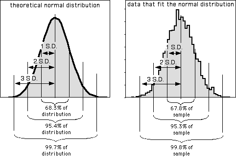
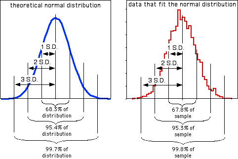
In addition to being more understandable than the variance as a measure of the amount of variation in the data, the standard deviation summarizes how close observations are to the mean in an understandable way. Many variables in biology fit the normal probability distribution fairly well. If a variable fits the normal distribution, 68.3% (or roughly two-thirds) of the values are within one standard deviation of the mean, 95.4% are within two standard deviations of the mean, and 99.7 (or almost all) are within 3 standard deviations of the mean. Thus if someone says the mean length of men's feet is 270 mm with a standard deviation of 13 mm, you know that about two-thirds of men's feet are between 257 and 283 mm long, and about 95% of men's feet are between 244 and 296 mm long. Here's a histogram that illustrates this:

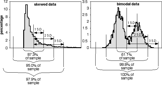
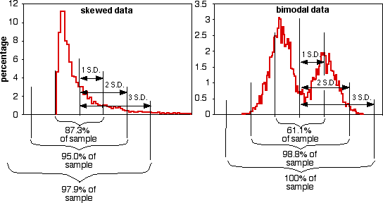
The proportions of the data that are within 1, 2, or 3 standard deviations of the mean are different if the data do not fit the normal distribution, as shown for these two very non-normal data sets:

Coefficient of variation. Coefficient of variation is the standard deviation divided by the mean; it summarizes the amount of variation as a percentage or proportion of the total. It is useful when comparing the amount of variation for one variable among groups with different means, or among different measurement variables. For example, the United States military measured foot length and foot width in 1774 American men. The standard deviation of foot length was 13.1 mm and the standard deviation for foot width was 5.26 mm, which makes it seem as if foot length is more variable than foot width. However, feet are longer than they are wide. Dividing by the means (269.7 mm for length, 100.6 mm for width), the coefficients of variation is actually slightly smaller for length (4.9%) than for width (5.2%), which for most purposes would be a more useful measure of variation.
Example
Here are the statistics of dispersion for the blacknose dace data from the central tendency web page. In reality, you would rarely have any reason to report all of these:
Range                      90
Variance                 1029.5
Standard deviation         32.09
Coefficient of variation   45.8%
How to calculate the statistics
Spreadsheet
I have made a spreadsheet that calculates the range, sample variance, sample standard deviation (with or without the Gurland and Tripathi correction), and coefficient of variation, for up to 1000 observations.
Web pages
This web page calculates standard deviation and other descriptive statistics for up to 10000 observations.
This web page calculates range, variance, and standard deviation, along with other descriptive statistics. I don't know the maximum number of observations it can handle.
R
Salvatore Mangiafico's R Companion has a sample R program for calculating range, sample variance, standard deviation, and coefficient of variation.
SAS
PROC UNIVARIATE will calculate the range, variance, standard deviation (without the Gurland and Tripathi correction), and coefficient of variation. It calculates the sample variance and sample standard deviation. For examples, see the central tendency web page.
Reference
Briones-Fourzán, P., and E. Lozano-Alvarez. 1991. Aspects of the biology of the giant isopod Bathynomus giganteus A. Milne Edwards, 1879 (Flabellifera: Cirolanidae), off the Yucatan Peninsula. Journal of Crustacean Biology 11: 375-385.
Gurland, J., and R.C. Tripathi. 1971. A simple approximation for unbiased estimation of the standard deviation. American Statistician 25: 30-32.
⇐ Previous topic|Next topic ⇒
Table of Contents
This page was last revised July 20, 2015. Its address is http://www.biostathandbook.com/dispersion.html. It may be cited as:
McDonald, J.H. 2014. Handbook of Biological Statistics (3rd ed.). Sparky House Publishing, Baltimore, Maryland. This web page contains the content of pages 107-110 in the printed version.
©2014 by John H. McDonald. You can probably do what you want with this content; see the permissions page for details.


