
⇐ Previous topic|Next topic
⇒
Table of Contents
Small numbers in chi-square and G–tests
Summary
Chi-square and G–tests are somewhat inaccurate when expected numbers are small, and you should use exact tests instead. I suggest a much higher definition of "small" than other people.
The problem with small numbers
Chi-square and G–tests of goodness-of-fit or independence give inaccurate results when the expected numbers are small. For example, let's say you want to know whether right-handed people tear the anterior cruciate ligament (ACL) in their right knee more or less often than the left ACL. You find 11 people with ACL tears, so your expected numbers (if your null hypothesis is true) are 5.5 right ACL tears and 5.5 left ACL tears. Let's say you actually observe 9 right ACL tears and 2 left ACL tears. If you compare the observed numbers to the expected using the exact test of goodness-of-fit, you get a P value of 0.065; the chi-square test of goodness-of-fit gives a P value of 0.035, and the G–test of goodness-of-fit gives a P value of 0.028. If you analyzed the data using the chi-square or G–test, you would conclude that people tear their right ACL significantly more than their left ACL; if you used the exact binomial test, which is more accurate, the evidence would not be quite strong enough to reject the null hypothesis.
When the sample sizes are too small, you should use exact tests instead of the chi-square test or G–test. However, how small is "too small"? The conventional rule of thumb is that if all of the expected numbers are greater than 5, it's acceptable to use the chi-square or G–test; if an expected number is less than 5, you should use an alternative, such as an exact test of goodness-of-fit or a Fisher's exact test of independence.
This rule of thumb is left over from the olden days, when the calculations necessary for an exact test were exceedingly tedious and error-prone. Now that we have these new-fangled gadgets called computers, it's time to retire the "no expected values less than 5" rule. But what new rule should you use?
Here is a graph of relative P values versus sample size. For each sample size, I found a pair of numbers that would give a P value for the exact test of goodness-of-fit (null hypothesis, 1:1 ratio) that was as close as possible to P=0.05 without going under it. For example, with a sample size of 11, the numbers 9 and 2 give a P value of 0.065. I did the chi-square test on these numbers, and I divided the chi-square P value by the exact binomial P value. For 9 and 2, the chi-square P value is 0.035, so the ratio is 0.035/0.065 = 0.54. In other words, the chi-square test gives a P value that is only 54% as large as the more accurate exact test. The G–test gives almost the same results as the chi-square test.
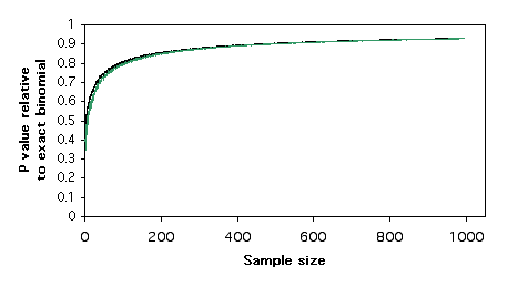
Plotting these relative P values vs. sample size , it is clear that the chi-square and G–tests give P values that are too low, even for sample sizes in the hundreds. This means that if you use a chi-square or G–test of goodness-of-fit and the P value is just barely significant, you will reject the null hypothesis, even though the more accurate P value of the exact binomial test would be above 0.05. The results are similar for 2×2 tests of independence; the chi-square and G–tests give P values that are considerably lower than that of the more accurate Fisher's exact test.
Yates' and William's corrections
One solution to this problem is to use Yates' correction for continuity, sometimes just known as the continuity correction. To do this, you subtract 0.5 from each observed value that is greater than the expected, add 0.5 to each observed value that is less than the expected, then do the chi-square or G–test. This only applies to tests with one degree of freedom: goodness-of-fit tests with only two categories, and 2×2 tests of independence. It works quite well for goodness-of-fit, yielding P values that are quite close to those of the exact binomial. For tests of independence, Yates' correction yields P values that are too high.
Another correction that is sometimes used is Williams' correction. For a goodness-of-fit test, Williams' correction is found by dividing the chi-square or G values by the following:
q=1+(a2−1)/(6nv)
where a is the number of categories, n is the total sample size, and v is the number of degrees of freedom. For a test of independence with R rows and C columns, Williams' correction is found by dividing the chi-square or G value by the following:
q=1+(n{[1/(row 1 total)]+…+[1/(row R total)]}−1)(n{[1/(column 1 total)]+…[1/(column C total)]}−1)/ [6n(R−1)(C−1)]
Unlike Yates' correction, it can be applied to tests with more than one degree of freedom. For the numbers I've tried, it increases the P value a little, but not enough to make it very much closer to the more accurate P value provided by the exact test of goodness-of-fit or Fisher's exact test.
Some software may apply the Yates' or Williams' correction automatically. When reporting your results, be sure to say whether or not you used one of these corrections.
Pooling
When a variable has more than two categories, and some of them have small numbers, it often makes sense to pool some of the categories together. For example, let's say you want to compare the proportions of different kinds of ankle injuries in basketball players vs. volleyball players, and your numbers look like this:
| basketball | volleyball | |
|---|---|---|
| sprains | 18 | 16 |
| breaks | 13 | 5 |
| torn ligaments | 9 | 7 |
| cuts | 3 | 5 |
| puncture wounds | 1 | 3 |
| infections | 2 | 0 |
The numbers for cuts, puncture wounds, and infections are pretty small, and this will cause the P value for your test of independence to be inaccurate. Having a large number of categories with small numbers will also decrease the power of your test to detect a significant difference; adding categories with small numbers can't increase the chi-square value or G-value very much, but it does increase the degrees of freedom. It would therefore make sense to pool some categories:
| basketball | volleyball | |
|---|---|---|
| sprains | 18 | 16 |
| breaks | 13 | 5 |
| torn ligaments | 9 | 7 |
| other injuries | 6 | 8 |
Depending on the biological question you're interested in, it might make sense to pool the data further:
| basketball | volleyball | |
|---|---|---|
| orthopedic injuries | 40 | 28 |
| non-orthopedic injuries | 6 | 8 |
It is important to make decisions about pooling before analyzing the data. In this case, you might have known, based on previous studies, that cuts, puncture wounds, and infections would be relatively rare and should be pooled. You could have decided before the study to pool all injuries for which the total was 10 or fewer, or you could have decided to pool all non-orthopedic injuries because they're just not biomechanically interesting.
Recommendation
I recommend that you always use an exact test (exact test of goodness-of-fit, Fisher's exact test) if the total sample size is less than 1000. There is nothing magical about a sample size of 1000, it's just a nice round number that is well within the range where an exact test, chi-square test and G–test will give almost identical P values. Spreadsheets, web-page calculators, and SAS shouldn't have any problem doing an exact test on a sample size of 1000.
When the sample size gets much larger than 1000, even a powerful program such as SAS on a mainframe computer may have problems doing the calculations needed for an exact test, so you should use a chi-square or G–test for sample sizes larger than this. You can use Yates' correction if there is only one degree of freedom, but with such a large sample size, the improvement in accuracy will be trivial.
For simplicity, I base my rule of thumb on the total sample size, not the smallest expected value; if one or more of your expected values are quite small, you should still try an exact test even if the total sample size is above 1000, and hope your computer can handle the calculations.
If you see someone else following the traditional rules and using chi-square or G–tests for total sample sizes that are smaller than 1000, don't worry about it too much. Old habits die hard, and unless their expected values are really small (in the single digits), it probably won't make any difference in the conclusions. If their chi-square or G–test gives a P value that's just a little below 0.05, you might want to analyze their data yourself, and if an exact test brings the P value above 0.05, you should probably point this out.
If you have a large number of categories, some with very small expected numbers, you should consider pooling the rarer categories, even if the total sample size is small enough to do an exact test; the fewer numbers of degrees of freedom will increase the power of your test.
⇐ Previous topic|Next topic
⇒
Table of Contents
This page was last revised December 4, 2014. Its address is http://www.biostathandbook.com/small.html. It may be cited as:
McDonald, J.H. 2014. Handbook of Biological Statistics (3rd ed.). Sparky House Publishing, Baltimore, Maryland. This web page contains the content of pages 86-89 in the printed version.
©2014 by John H. McDonald. You can probably do what you want with this content; see the permissions page for details.