Search the handbook:

⇐ Previous topic|Next topic ⇒
Table of Contents

---

Confidence limits

---

Summary

Confidence limits tell you how accurate your estimate of the mean is likely to be.

Introduction

After you've calculated the mean of a set of observations, you should give some indication of how close your estimate is likely to be to the parametric ("true") mean. One way to do this is with confidence limits. Confidence limits are the numbers at the upper and lower end of a confidence interval; for example, if your mean is 7.4 with confidence limits of 5.4 and 9.4, your confidence interval is 5.4 to 9.4. Most people use 95% confidence limits, although you could use other values. Setting 95% confidence limits means that if you took repeated random samples from a population and calculated the mean and confidence limits for each sample, the confidence interval for 95% of your samples would include the parametric mean.

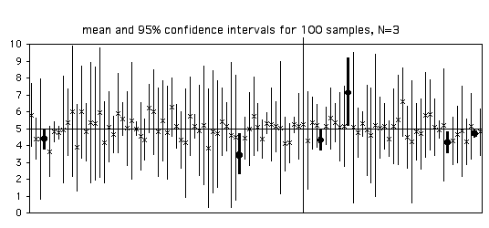
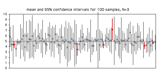
To illustrate this, here are the means and confidence intervals for 100 samples of 3 observations from a population with a parametric mean of 5. Of the 100 samples, 94 (shown with X for the mean and a thin line for the confidence interval) have the parametric mean within their 95% confidence interval, and 6 (shown with circles and thick lines) have the parametric mean outside the confidence interval.

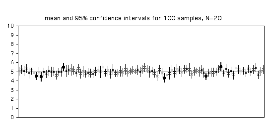
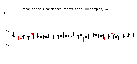
With larger sample sizes, the 95% confidence intervals get smaller:

When you calculate the confidence interval for a single sample, it is tempting to say that "there is a 95% probability that the confidence interval includes the parametric mean." This is technically incorrect, because it implies that if you collected samples with the same confidence interval, sometimes they would include the parametric mean and sometimes they wouldn't. For example, the first sample in the figure above has confidence limits of 4.59 and 5.51. It would be incorrect to say that 95% of the time, the parametric mean for this population would lie between 4.59 and 5.51. If you took repeated samples from this same population and repeatedly got confidence limits of 4.59 and 5.51, the parametric mean (which is 5, remember) would be in this interval 100% of the time. Some statisticians don't care about this confusing, pedantic distinction, but others are very picky about it, so it's good to know.

Confidence limits for measurement variables

To calculate the confidence limits for a measurement variable, multiply the standard error of the mean times the appropriate t-value. The t-value is determined by the probability (0.05 for a 95% confidence interval) and the degrees of freedom (n−1). In a spreadsheet, you could use =(STDEV(Ys)/SQRT(COUNT(Ys)))*TINV(0.05, COUNT(Ys)-1), where Ys is the range of cells containing your data. You add this value to and subtract it from the mean to get the confidence limits. Thus if the mean is 87 and the t-value times the standard error is 10.3, the confidence limits would be 76.7 and 97.3. You could also report this as "87 ±10.3 (95% confidence limits)." People report both confidence limits and standard errors as the "mean ± something," so always be sure to specify which you're talking about.

All of the above applies only to normally distributed measurement variables. For measurement data from a highly non-normal distribution, bootstrap techniques, which I won't talk about here, might yield better estimates of the confidence limits.

Confidence limits for nominal variables

There is a different, more complicated formula, based on the binomial distribution, for calculating confidence limits of proportions (nominal data). Importantly, it yields confidence limits that are not symmetrical around the proportion, especially for proportions near zero or one. John Pezzullo has an easy-to-use web page for confidence intervals of a proportion. To see how it works, let's say that you've taken a sample of 20 men and found 2 colorblind and 18 non-colorblind. Go to the web page and enter 2 in the "Numerator" box and 20 in the "Denominator" box," then hit "Compute." The results for this example would be a lower confidence limit of 0.0124 and an upper confidence limit of 0.3170. You can't report the proportion of colorblind men as "0.10 ± something," instead you'd have to say "0.10 with 95% confidence limits of 0.0124 and 0.3170."

An alternative technique for estimating the confidence limits of a proportion assumes that the sample proportions are normally distributed. This approximate technique yields symmetrical confidence limits, which for proportions near zero or one are obviously incorrect. For example, if you calculate the confidence limits using the normal approximation on 0.10 with a sample size of 20, you get -0.03 and 0.23, which is ridiculous (you couldn't have less than 0% of men being color-blind). It would also be incorrect to say that the confidence limits were 0 and 0.23, because you know the proportion of colorblind men in your population is greater than 0 (your sample had two colorblind men, so you know the population has at least two colorblind men). I consider confidence limits for proportions that are based on the normal approximation to be obsolete for most purposes; you should use the confidence interval based on the binomial distribution, unless the sample size is so large that it is computationally impractical. Unfortunately, more people use the confidence limits based on the normal approximation than use the correct, binomial confidence limits.

The formula for the 95% confidence interval using the normal approximation is p ±1.96√[p(1-p)/n], where p is the proportion and n is the sample size. Thus, for P=0.20 and n=100, the confidence interval would be ±1.96√[0.20(1-0.20)/100], or 0.20±0.078. A common rule of thumb says that it is okay to use this approximation as long as npq is greater than 5; my rule of thumb is to only use the normal approximation when the sample size is so large that calculating the exact binomial confidence interval makes smoke come out of your computer.

Statistical testing with confidence intervals

This handbook mostly presents "classical" or "frequentist" statistics, in which hypotheses are tested by estimating the probability of getting the observed results by chance, if the null is true (the P value). An alternative way of doing statistics is to put a confidence interval on a measure of the deviation from the null hypothesis. For example, rather than comparing two means with a two-sample t–test, some statisticians would calculate the confidence interval of the difference in the means.

This approach is valuable if a small deviation from the null hypothesis would be uninteresting, when you're more interested in the size of the effect rather than whether it exists. For example, if you're doing final testing of a new drug that you're confident will have some effect, you'd be mainly interested in estimating how well it worked, and how confident you were in the size of that effect. You'd want your result to be "This drug reduced systolic blood pressure by 10.7 mm Hg, with a confidence interval of 7.8 to 13.6," not "This drug significantly reduced systolic blood pressure (P=0.0007)."

Using confidence limits this way, as an alternative to frequentist statistics, has many advocates, and it can be a useful approach. However, I often see people saying things like "The difference in mean blood pressure was 10.7 mm Hg, with a confidence interval of 7.8 to 13.6; because the confidence interval on the difference does not include 0, the means are significantly different." This is just a clumsy, roundabout way of doing hypothesis testing, and they should just admit it and do a frequentist statistical test.

There is a myth that when two means have confidence intervals that overlap, the means are not significantly different (at the P<0.05 level). Another version of this myth is that if each mean is outside the confidence interval of the other mean, the means are significantly different. Neither of these is true (Schenker and Gentleman 2001, Payton et al. 2003); it is easy for two sets of numbers to have overlapping confidence intervals, yet still be significantly different by a two-sample t–test; conversely, each mean can be outside the confidence interval of the other, yet they're still not significantly different. Don't try compare two means by visually comparing their confidence intervals, just use the correct statistical test.

Similar statistics

Confidence limits and standard error of the mean serve the same purpose, to express the reliability of an estimate of the mean. When you look at scientific papers, sometimes the "error bars" on graphs or the ± number after means in tables represent the standard error of the mean, while in other papers they represent 95% confidence intervals. I prefer 95% confidence intervals. When I see a graph with a bunch of points and error bars representing means and confidence intervals, I know that most (95%) of the error bars include the parametric means. When the error bars are standard errors of the mean, only about two-thirds of the bars are expected to include the parametric means; I have to mentally double the bars to get the approximate size of the 95% confidence interval (because t(0.05) is approximately 2 for all but very small values of n). Whichever statistic you decide to use, be sure to make it clear what the error bars on your graphs represent. A surprising number of papers don't say what their error bars represent, which means that the only information the error bars convey to the reader is that the authors are careless and sloppy.

Examples

Measurement data: The blacknose dace data from the central tendency web page has an arithmetic mean of 70.0. The lower confidence limit is 45.3 (70.0−24.7), and the upper confidence limit is 94.7 (70+24.7).

Nominal data: If you work with a lot of proportions, it's good to have a rough idea of confidence limits for different sample sizes, so you have an idea of how much data you'll need for a particular comparison. For proportions near 50%, the confidence intervals are roughly ±30%, 10%, 3%, and 1% for n=10, 100, 1000, and 10,000, respectively. This is why the "margin of error" in political polls, which typically have a sample size of around 1,000, is usually about 3%. Of course, this rough idea is no substitute for an actual power analysis.

n	proportion=0.10	proportion=0.50
10	0.0025, 0.4450	0.1871, 0.8129
100	0.0490, 0.1762	0.3983, 0.6017
1000	0.0821, 0.1203	0.4685, 0.5315
10,000	0.0942, 0.1060	0.4902, 0.5098

How to calculate confidence limits

Spreadsheets

The descriptive statistics spreadsheet calculates 95% confidence limits of the mean for up to 1000 measurements. The confidence intervals for a binomial proportion spreadsheet calculates 95% confidence limits for nominal variables, using both the exact binomial and the normal approximation.

Web pages

This web page calculates confidence intervals of the mean for up to 10,000 measurement observations. The web page for confidence intervals of a proportion handles nominal variables.

R

Salvatore Mangiafico's R Companion has sample R programs for confidence limits for both measurement and nominal variables.

SAS

To get confidence limits for a measurement variable, add CIBASIC to the PROC UNIVARIATE statement, like this:

data fish;
   input location $ dacenumber;
   cards;
Mill_Creek_1               76
Mill_Creek_2              102
North_Branch_Rock_Creek_1  12
North_Branch_Rock_Creek_2  39
Rock_Creek_1               55
Rock_Creek_2               93
Rock_Creek_3               98
Rock_Creek_4               53
Turkey_Branch             102
;
proc univariate data=fish cibasic;
run;

The output will include the 95% confidence limits for the mean (and for the standard deviation and variance, which you would hardly ever need):

       Basic Confidence Limits Assuming Normality
 
   Parameter          Estimate     95% Confidence Limits

   Mean               70.00000      45.33665    94.66335
   Std Deviation      32.08582      21.67259    61.46908
   Variance               1030     469.70135        3778

This shows that the blacknose dace data have a mean of 70, with confidence limits of 45.3 and 94.7.

You can get the confidence limits for a binomial proportion using PROC FREQ. Here's the sample program from the exact test of goodness-of-fit page:

 
data gus;
   input paw $;
   cards;
right
left
right
right
right
right
left
right
right
right
;
proc freq data=gus;
   tables paw / binomial(P=0.5);
exact binomial;
run;

And here is part of the output:

         Binomial Proportion
            for paw = left
   --------------------------------
   Proportion                0.2000
   ASE                       0.1265
   95% Lower Conf Limit      0.0000
   95% Upper Conf Limit      0.4479

   Exact Conf Limits               
   95% Lower Conf Limit      0.0252
   95% Upper Conf Limit      0.5561

The first pair of confidence limits shown is based on the normal approximation; the second pair is the better one, based on the exact binomial calculation. Note that if you have more than two values of the nominal variable, the confidence limits will only be calculated for the value whose name is first alphabetically. For example, if the Gus data set included "left," "right," and "both" as values, SAS would only calculate the confidence limits on the proportion of "both." One clumsy way to solve this would be to run the program three times, changing the name of "left" to "aleft," then changing the name of "right" to "aright," to make each one first in one run.

References

Payton, M. E., M. H. Greenstone, and N. Schenker. 2003. Overlapping confidence intervals or standard error intervals: what do they mean in terms of statistical significance? Journal of Insect Science 3: 34.

Schenker, N., and J. F. Gentleman. 2001. On judging the significance of differences by examining overlap between confidence intervals. American Statistician 55: 182-186.

---

⇐ Previous topic|Next topic ⇒
Table of Contents

---

This page was last revised July 20, 2015. Its address is http://www.biostathandbook.com/confidence.html. It may be cited as:
McDonald, J.H. 2014. Handbook of Biological Statistics (3rd ed.). Sparky House Publishing, Baltimore, Maryland. This web page contains the content of pages 115-120 in the printed version.

©2014 by John H. McDonald. You can probably do what you want with this content; see the permissions page for details.