
⇐ Previous topic|Next topic ⇒
Table of Contents
Two-way anova
Summary
Use two-way anova when you have one measurement variable and two nominal variables, and each value of one nominal variable is found in combination with each value of the other nominal variable. It tests three null hypotheses: that the means of the measurement variable are equal for different values of the first nominal variable; that the means are equal for different values of the second nominal variable; and that there is no interaction (the effects of one nominal variable don't depend on the value of the other nominal variable).
When to use it
You use a two-way anova (also known as a factorial anova, with two factors) when you have one measurement variable and two nominal variables. The nominal variables (often called "factors" or "main effects") are found in all possible combinations.
For example, here's some data I collected on the enzyme activity of mannose-6-phosphate isomerase (MPI) and MPI genotypes in the amphipod crustacean Platorchestia platensis. Because I didn't know whether sex also affected MPI activity, I separated the amphipods by sex.
| Genotype | Female | Male |
|---|---|---|
| FF | 2.838 4.216 2.889 4.198 | 1.884 2.283 4.939 3.486 |
| FS | 3.55 4.556 3.087 1.943 | 2.396 2.956 3.105 2.649 |
| SS | 3.620 3.079 3.586 2.669 | 2.801 3.421 4.275 3.110 |
Unlike a nested anova, each grouping extends across the other grouping: each genotype contains some males and some females, and each sex contains all three genotypes.
A two-way anova is usually done with replication (more than one observation for each combination of the nominal variables). For our amphipods, a two-way anova with replication means there are more than one male and more than one female of each genotype. You can also do two-way anova without replication (only one observation for each combination of the nominal variables), but this is less informative (you can't test the interaction term) and requires you to assume that there is no interaction.
Repeated measures: One experimental design that people analyze with a two-way anova is repeated measures, where an observation has been made on the same individual more than once. This usually involves measurements taken at different time points. For example, you might measure running speed before, one week into, and three weeks into a program of exercise. Because individuals would start with different running speeds, it is better to analyze using a two-way anova, with "individual" as one of the factors, rather than lumping everyone together and analyzing with a one-way anova. Sometimes the repeated measures are repeated at different places rather than different times, such as the hip abduction angle measured on the right and left hip of individuals. Repeated measures experiments are often done without replication, although they could be done with replication.
In a repeated measures design, one of main effects is usually uninteresting and the test of its null hypothesis may not be reported. If the goal is to determine whether a particular exercise program affects running speed, there would be little point in testing whether individuals differed from each other in their average running speed; only the change in running speed over time would be of interest.
Randomized blocks: Another experimental design that is analyzed by a two-way anova is randomized blocks. This often occurs in agriculture, where you may want to test different treatments on small plots within larger blocks of land. Because the larger blocks may differ in some way that may affect the measurement variable, the data are analyzed with a two-way anova, with the block as one of the nominal variables. Each treatment is applied to one or more plot within the larger block, and the positions of the treatments are assigned at random. This is most commonly done without replication (one plot per block), but it can be done with replication as well.
Null hypotheses
A two-way anova with replication tests three null hypotheses: that the means of observations grouped by one factor are the same; that the means of observations grouped by the other factor are the same; and that there is no interaction between the two factors. The interaction test tells you whether the effects of one factor depend on the other factor. In the amphipod example, imagine that female amphipods of each genotype have about the same MPI activity, while male amphipods with the SS genotype had much lower MPI activity than male FF or FS amphipods (they don't, but imagine they do for a moment). The different effects of genotype on activity in female and male amphipods would result in a significant interaction term in the anova, meaning that the effect of genotype on activity would depend on whether you were looking at males or females. If there were no interaction, the differences among genotypes in enzyme activity would be the same for males and females, and the difference in activity between males and females would be the same for each of the three genotypes.
When the interaction term is significant, the usual advice is that you should not test the effects of the individual factors. In this example, it would be misleading to examine the individual factors and conclude "SS amphipods have lower activity than FF or FS," when that is only true for males, or "Male amphipods have lower MPI activity than females," when that is only true for the SS genotype.
What you can do, if the interaction term is significant, is look at each factor separately, using a one-way anova. In the amphipod example, you might be able to say that for female amphipods, there is no significant effect of genotype on MPI activity, while for male amphipods, there is a significant effect of genotype on MPI activity. Or, if you're more interested in the sex difference, you might say that male amphipods have a significantly lower mean enzyme activity than females when they have the SS genotype, but not when they have the other two genotypes.
When you do a two-way anova without replication, you can still test the two main effects, but you can't test the interaction. This means that your tests of the main effects have to assume that there's no interaction. If you find a significant difference in the means for one of the main effects, you wouldn't know whether that difference was consistent for different values of the other main effect.
How the test works
With replication
When the sample sizes in each subgroup are equal (a "balanced design"), you calculate the mean square for each of the two factors (the "main effects"), for the interaction, and for the variation within each combination of factors. You then calculate each F-statistic by dividing a mean square by the within-subgroup mean square.
When the sample sizes for the subgroups are not equal (an "unbalanced design"), the analysis is much more complicated, and there are several different techniques for testing the main and interaction effects that I'm not going to cover here. If you're doing a two-way anova, your statistical life will be a lot easier if you make it a balanced design.
Without replication
When there is only a single observation for each combination of the nominal variables, there are only two null hypotheses: that the means of observations grouped by one factor are the same, and that the means of observations grouped by the other factor are the same. It is impossible to test the null hypothesis of no interaction; instead, you have to assume that there is no interaction in order to test the two main effects.
When there is no replication, you calculate the mean square for each of the two main effects, and you also calculate a total mean square by considering all of the observations as a single group. The remainder mean square (also called the discrepance or error mean square) is found by subtracting the two main effect mean squares from the total mean square. The F-statistic for a main effect is the main effect mean square divided by the remainder mean square.
Assumptions
Two-way anova, like all anovas, assumes that the observations within each cell are normally distributed and have equal standard deviations. I don't know how sensitive it is to violations of these assumptions.
Examples
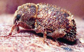
Shimoji and Miyatake (2002) raised the West Indian sweetpotato weevil for 14 generations on an artificial diet. They compared these artificial diet weevils (AD strain) with weevils raised on sweet potato roots (SP strain), the weevil's natural food. They placed multiple females of each strain on either the artificial diet or sweet potato root, and they counted the number of eggs each female laid over a 28-day period. There are two nominal variables, the strain of weevil (AD or SP) and the oviposition test food (artificial diet or sweet potato), and one measurement variable (the number of eggs laid).
The results of the two-way anova with replication include a significant interaction term (F1, 117=17.02, P=7 x 10⁻⁵). Looking at the graph, the interaction can be interpreted this way: on the sweet potato diet, the SP strain laid more eggs than the AD strain; on the artificial diet, the AD strain laid more eggs than the SP strain. Each main effect is also significant: weevil strain (F1, 117=8.82, P=0.0036) and oviposition test food (F=1, 117=345.92, P=9 x 10-37). However, the significant effect of strain is a bit misleading, as the direction of the difference between strains depends on which food they ate. This is why it is important to look at the interaction term first.
Place and Abramson (2008) put diamondback rattlesnakes (Crotalus atrox) in a "rattlebox," a box with a lid that would slide open and shut every 5 minutes. At first, the snake would rattle its tail each time the box opened. After a while, the snake would become habituated to the box opening and stop rattling its tail. They counted the number of box openings until a snake stopped rattling; fewer box openings means the snake was more quickly habituated. They repeated this experiment on each snake on four successive days, which I'll treat as a nominal variable for this example. Place and Abramson (2008) used 10 snakes, but some of them never became habituated; to simplify this example, I'll use data from the 6 snakes that did become habituated on each day:
| Snake ID | Day 1 | Day 2 | Day 3 | Day 4 |
|---|---|---|---|---|
| D1 | 85 | 58 | 15 | 57 |
| D3 | 107 | 51 | 30 | 12 |
| D5 | 61 | 60 | 68 | 36 |
| D8 | 22 | 41 | 63 | 21 |
| D11 | 40 | 45 | 28 | 10 |
| D12 | 65 | 27 | 3 | 16 |
The measurement variable is trials to habituation, and the two nominal variables are day (1 to 4) and snake ID. This is a repeated measures design, as the measurement variable is measured repeatedly on each snake. It is analyzed using a two-way anova without replication. The effect of snake is not significant (F5, 15=1.24, P=0.34), while the effect of day is significant (F3, 15=3.32, P=0.049).
Graphing the results
Some people plot the results of a two-way anova on a 3-D graph, with the measurement variable on the Y axis, one nominal variable on the X-axis, and the other nominal variable on the Z axis (going into the paper). This makes it difficult to visually compare the heights of the bars in the front and back rows, so I don't recommend this. Instead, I suggest you plot a bar graph with the bars clustered by one nominal variable, with the other nominal variable identified using the color or pattern of the bars.
If one of the nominal variables is the interesting one, and the other is just a possible confounder, I'd group the bars by the possible confounder and use different patterns for the interesting variable. For the amphipod data described above, I was interested in seeing whether MPI phenotype affected enzyme activity, with any difference between males and females as an annoying confounder, so I grouped the bars by sex.
Similar tests
A two-way anova without replication and only two values for the interesting nominal variable may be analyzed using a paired t–test. The results of a paired t–test are mathematically identical to those of a two-way anova, but the paired t–test is easier to do and is familiar to more people. Data sets with one measurement variable and two nominal variables, with one nominal variable nested under the other, are analyzed with a nested anova.
Three-way and higher order anovas are possible, as are anovas combining aspects of a nested and a two-way or higher order anova. The number of interaction terms increases rapidly as designs get more complicated, and the interpretation of any significant interactions can be quite difficult. It is better, when possible, to design your experiments so that as many factors as possible are controlled, rather than collecting a hodgepodge of data and hoping that a sophisticated statistical analysis can make some sense of it.
How to do the test
Spreadsheet
I haven't put together a spreadsheet to do two-way anovas.
Web page
There's a web page to perform a two-way anova with replication, with up to 4 groups for each main effect.
R
Salvatore Mangiafico's R Companion has a sample R program for two-way anova.
SAS
Use PROC GLM for a two-way anova. The CLASS statement lists the two nominal variables. The MODEL statement has the measurement variable, then the two nominal variables and their interaction after the equals sign. Here is an example using the MPI activity data described above:
DATA amphipods;
   INPUT id $ sex $ genotype $ activity @@;
   DATALINES;
 1 male   ff 1.884   2  male   ff 2.283   3  male   fs 2.396   4  female ff 2.838
 5 male   fs 2.956   6  female ff 4.216   7  female ss 3.620   8  female ff 2.889
 9 female fs 3.550  10  male   fs 3.105  11  female fs 4.556  12  female fs 3.087
13 male   ff 4.939  14  male   ff 3.486  15  female ss 3.079  16  male   fs 2.649
17 female fs 1.943  19  female ff 4.198  20  female ff 2.473  22  female ff 2.033
24 female fs 2.200  25  female fs 2.157  26  male   ss 2.801  28  male   ss 3.421
29 female ff 1.811  30  female fs 4.281  32  female fs 4.772  34  female ss 3.586
36 female ff 3.944  38  female ss 2.669  39  female ss 3.050  41  male   ss 4.275
43 female ss 2.963  46  female ss 3.236  48  female ss 3.673  49  male   ss 3.110
;
PROC GLM DATA=amphipods;
  CLASS sex genotype;
  MODEL activity=sex genotype sex*genotype;
RUN;
The results indicate that the interaction term is not significant (P=0.60), the effect of genotype is not significant (P=0.84), and the effect of sex concentration not significant (P=0.77).
Source        DF     Type I SS    Mean Square   F Value    Pr > F

sex            1    0.06808050     0.06808050      0.09    0.7712
genotype       2    0.27724017     0.13862008      0.18    0.8400
sex*genotype   2    0.81464133     0.40732067      0.52    0.6025
If you are using SAS to do a two-way anova without replication, do not put an interaction term in the model statement (sex*genotype is the interaction term in the example above).
References
Place, A.J., and C.I. Abramson. 2008. Habituation of the rattle response in western diamondback rattlesnakes, Crotalus atrox. Copeia 2008: 835-843.
Shimoji, Y., and T. Miyatake. 2002. Adaptation to artificial rearing during successive generations in the West Indian sweetpotato weevil, Euscepes postfasciatus (Coleoptera: Curuculionidae). Annals of the Entomological Society of America 95: 735-739.
⇐ Previous topic|Next topic ⇒
Table of Contents
This page was last revised July 20, 2015. Its address is http://www.biostathandbook.com/twowayanova.html. It may be cited as:
McDonald, J.H. 2014. Handbook of Biological Statistics (3rd ed.). Sparky House Publishing, Baltimore, Maryland. This web page contains the content of pages 173-179 in the printed version.
©2014 by John H. McDonald. You can probably do what you want with this content; see the permissions page for details.