Search the handbook:

⇐ Previous topic|Next topic ⇒
Table of Contents

---

Kruskal–Wallis test

---

Summary

Use the Kruskal–Wallis test when you have one nominal variable and one ranked variable. It tests whether the mean ranks are the same in all the groups.

When to use it

The most common use of the Kruskal–Wallis test is when you have one nominal variable and one measurement variable, an experiment that you would usually analyze using one-way anova, but the measurement variable does not meet the normality assumption of a one-way anova. Some people have the attitude that unless you have a large sample size and can clearly demonstrate that your data are normal, you should routinely use Kruskal–Wallis; they think it is dangerous to use one-way anova, which assumes normality, when you don't know for sure that your data are normal. However, one-way anova is not very sensitive to deviations from normality. I've done simulations with a variety of non-normal distributions, including flat, highly peaked, highly skewed, and bimodal, and the proportion of false positives is always around 5% or a little lower, just as it should be. For this reason, I don't recommend the Kruskal-Wallis test as an alternative to one-way anova. Because many people use it, you should be familiar with it even if I convince you that it's overused.

The Kruskal-Wallis test is a non-parametric test, which means that it does not assume that the data come from a distribution that can be completely described by two parameters, mean and standard deviation (the way a normal distribution can). Like most non-parametric tests, you perform it on ranked data, so you convert the measurement observations to their ranks in the overall data set: the smallest value gets a rank of 1, the next smallest gets a rank of 2, and so on. You lose information when you substitute ranks for the original values, which can make this a somewhat less powerful test than a one-way anova; this is another reason to prefer one-way anova.

The other assumption of one-way anova is that the variation within the groups is equal (homoscedasticity). While Kruskal-Wallis does not assume that the data are normal, it does assume that the different groups have the same distribution, and groups with different standard deviations have different distributions. If your data are heteroscedastic, Kruskal–Wallis is no better than one-way anova, and may be worse. Instead, you should use Welch's anova for heteoscedastic data.

The only time I recommend using Kruskal-Wallis is when your original data set actually consists of one nominal variable and one ranked variable; in this case, you cannot do a one-way anova and must use the Kruskal–Wallis test. Dominance hierarchies (in behavioral biology) and developmental stages are the only ranked variables I can think of that are common in biology.

The Mann–Whitney U-test (also known as the Mann–Whitney–Wilcoxon test, the Wilcoxon rank-sum test, or the Wilcoxon two-sample test) is limited to nominal variables with only two values; it is the non-parametric analogue to two-sample t–test. It uses a different test statistic (U instead of the H of the Kruskal–Wallis test), but the P value is mathematically identical to that of a Kruskal–Wallis test. For simplicity, I will only refer to Kruskal–Wallis on the rest of this web page, but everything also applies to the Mann–Whitney U-test.

The Kruskal–Wallis test is sometimes called Kruskal–Wallis one-way anova or non-parametric one-way anova. I think calling the Kruskal–Wallis test an anova is confusing, and I recommend that you just call it the Kruskal–Wallis test.

Null hypothesis

The null hypothesis of the Kruskal–Wallis test is that the mean ranks of the groups are the same. The expected mean rank depends only on the total number of observations (for n observations, the expected mean rank in each group is (n+1)/2), so it is not a very useful description of the data; it's not something you would plot on a graph.

You will sometimes see the null hypothesis of the Kruskal–Wallis test given as "The samples come from populations with the same distribution." This is correct, in that if the samples come from populations with the same distribution, the Kruskal–Wallis test will show no difference among them. I think it's a little misleading, however, because only some kinds of differences in distribution will be detected by the test. For example, if two populations have symmetrical distributions with the same center, but one is much wider than the other, their distributions are different but the Kruskal–Wallis test will not detect any difference between them.

The null hypothesis of the Kruskal–Wallis test is not that the means are the same. It is therefore incorrect to say something like "The mean concentration of fructose is higher in pears than in apples (Kruskal–Wallis test, P=0.02)," although you will see data summarized with means and then compared with Kruskal–Wallis tests in many publications. The common misunderstanding of the null hypothesis of Kruskal-Wallis is yet another reason I don't like it.

The null hypothesis of the Kruskal–Wallis test is often said to be that the medians of the groups are equal, but this is only true if you assume that the shape of the distribution in each group is the same. If the distributions are different, the Kruskal–Wallis test can reject the null hypothesis even though the medians are the same. To illustrate this point, I made up these three sets of numbers. They have identical means (43.5), and identical medians (27.5), but the mean ranks are different (34.6, 27.5, and 20.4, respectively), resulting in a significant (P=0.025) Kruskal–Wallis test:

Group 1	Group 2	Group 3
1	10	19
2	11	20
3	12	21
4	13	22
5	14	23
6	15	24
7	16	25
8	17	26
9	18	27
46	37	28
47	58	65
48	59	66
49	60	67
50	61	68
51	62	69
52	63	70
53	64	71
342	193	72

How the test works

Here are some data on Wright's F_ST (a measure of the amount of geographic variation in a genetic polymorphism) in two populations of the American oyster, Crassostrea virginica. McDonald et al. (1996) collected data on F_ST for six anonymous DNA polymorphisms (variation in random bits of DNA of no known function) and compared the F_ST values of the six DNA polymorphisms to F_ST values on 13 proteins from Buroker (1983). The biological question was whether protein polymorphisms would have generally lower or higher F_ST values than anonymous DNA polymorphisms. McDonald et al. (1996) knew that the theoretical distribution of F_ST for two populations is highly skewed, so they analyzed the data with a Kruskal–Wallis test.

When working with a measurement variable, the Kruskal–Wallis test starts by substituting the rank in the overall data set for each measurement value. The smallest value gets a rank of 1, the second-smallest gets a rank of 2, etc. Tied observations get average ranks; in this data set, the two F_st values of -0.005 are tied for second and third, so they get a rank of 2.5.

gene	class	FST	Rank	Rank
CVJ5	DNA	-0.006	1
CVB1	DNA	-0.005	2.5
6Pgd	protein	-0.005		2.5
Pgi	protein	-0.002		4
CVL3	DNA	0.003	5
Est-3	protein	0.004		6
Lap-2	protein	0.006		7
Pgm-1	protein	0.015		8
Aat-2	protein	0.016		9.5
Adk-1	protein	0.016		9.5
Sdh	protein	0.024		11
Acp-3	protein	0.041		12
Pgm-2	protein	0.044		13
Lap-1	protein	0.049		14
CVL1	DNA	0.053	15
Mpi-2	protein	0.058		16
Ap-1	protein	0.066		17
CVJ6	DNA	0.095	18
CVB2m	DNA	0.116	19
Est-1	protein	0.163		20

You calculate the sum of the ranks for each group, then the test statistic, H. H is given by a rather formidable formula that basically represents the variance of the ranks among groups, with an adjustment for the number of ties. H is approximately chi-square distributed, meaning that the probability of getting a particular value of H by chance, if the null hypothesis is true, is the P value corresponding to a chi-square equal to H; the degrees of freedom is the number of groups minus 1. For the example data, the mean rank for DNA is 10.08 and the mean rank for protein is 10.68, H=0.043, there is 1 degree of freedom, and the P value is 0.84. The null hypothesis that the F_ST of DNA and protein polymorphisms have the same mean ranks is not rejected.

For the reasons given above, I think it would actually be better to analyze the oyster data with one-way anova. It gives a P value of 0.75, which fortunately would not change the conclusions of McDonald et al. (1996).

If the sample sizes are too small, H does not follow a chi-squared distribution very well, and the results of the test should be used with caution. N less than 5 in each group seems to be the accepted definition of "too small."

Assumptions

The Kruskal–Wallis test does NOT assume that the data are normally distributed; that is its big advantage. If you're using it to test whether the medians are different, it does assume that the observations in each group come from populations with the same shape of distribution, so if different groups have different shapes (one is skewed to the right and another is skewed to the left, for example, or they have different variances), the Kruskal–Wallis test may give inaccurate results (Fagerland and Sandvik 2009). If you're interested in any difference among the groups that would make the mean ranks be different, then the Kruskal–Wallis test doesn't make any assumptions.

Heteroscedasticity is one way in which different groups can have different shaped distributions. If the distributions are heteroscedastic, the Kruskal–Wallis test won't help you; instead, you should use Welch's t–test for two groups, or Welch's anova for more than two groups.

Examples

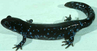
Bolek and Coggins (2003) collected multiple individuals of the toad Bufo americanus,, the frog Rana pipiens, and the salamander Ambystoma laterale from a small area of Wisconsin. They dissected the amphibians and counted the number of parasitic helminth worms in each individual. There is one measurement variable (worms per individual amphibian) and one nominal variable (species of amphibian), and the authors did not think the data fit the assumptions of an anova. The results of a Kruskal–Wallis test were significant (H=63.48, 2 d.f., P=1.6 X 10^-14); the mean ranks of worms per individual are significantly different among the three species.

---

Dog	Sex	Rank
Merlino	Male	1
Gastone	Male	2
Pippo	Male	3
Leon	Male	4
Golia	Male	5
Lancillotto	Male	6
Mamy	Female	7
Nanà	Female	8
Isotta	Female	9
Diana	Female	10
Simba	Male	11
Pongo	Male	12
Semola	Male	13
Kimba	Male	14
Morgana	Female	15
Stella	Female	16
Hansel	Male	17
Cucciola	Male	18
Mammolo	Male	19
Dotto	Male	20
Gongolo	Male	21
Gretel	Female	22
Brontolo	Female	23
Eolo	Female	24
Mag	Female	25
Emy	Female	26
Pisola	Female	27

Cafazzo et al. (2010) observed a group of free-ranging domestic dogs in the outskirts of Rome. Based on the direction of 1815 observations of submissive behavior, they were able to place the dogs in a dominance hierarchy, from most dominant (Merlino) to most submissive (Pisola). Because this is a true ranked variable, it is necessary to use the Kruskal–Wallis test. The mean rank for males (11.1) is lower than the mean rank for females (17.7), and the difference is significant (H=4.61, 1 d.f., P=0.032).

Graphing the results

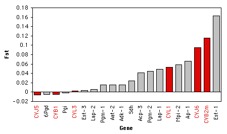
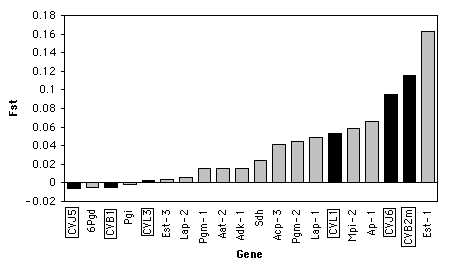
It is tricky to know how to visually display the results of a Kruskal–Wallis test. It would be misleading to plot the means or medians on a bar graph, as the Kruskal–Wallis test is not a test of the difference in means or medians. If there are relatively small number of observations, you could put the individual observations on a bar graph, with the value of the measurement variable on the Y axis and its rank on the X axis, and use a different pattern for each value of the nominal variable. Here's an example using the oyster F_st data:

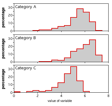
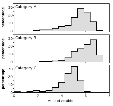
If there are larger numbers of observations, you could plot a histogram for each category, all with the same scale, and align them vertically. I don't have suitable data for this handy, so here's an illustration with imaginary data:

Similar tests

One-way anova is more powerful and a lot easier to understand than the Kruskal–Wallis test, so unless you have a true ranked variable, you should use it.

How to do the test

Spreadsheet

I have put together a spreadsheet to do the Kruskal–Wallis test on up to 20 groups, with up to 1000 observations per group.

Web pages

Richard Lowry has web pages for performing the Kruskal–Wallis test for two groups, three groups, or four groups.

R

Salvatore Mangiafico's R Companion has a sample R program for the Kruskal–Wallis test.

SAS

To do a Kruskal–Wallis test in SAS, use the NPAR1WAY procedure (that's the numeral "one," not the letter "el," in NPAR1WAY). WILCOXON tells the procedure to only do the Kruskal–Wallis test; if you leave that out, you'll get several other statistical tests as well, tempting you to pick the one whose results you like the best. The nominal variable that gives the group names is given with the CLASS parameter, while the measurement or ranked variable is given with the VAR parameter. Here's an example, using the oyster data from above:

DATA oysters;
 INPUT markername $ markertype $ fst;
 DATALINES;
CVB1   DNA      -0.005
CVB2m  DNA       0.116
CVJ5   DNA      -0.006
CVJ6   DNA       0.095
CVL1   DNA       0.053
CVL3   DNA       0.003
6Pgd   protein  -0.005
Aat-2  protein   0.016
Acp-3  protein   0.041
Adk-1  protein   0.016
Ap-1   protein   0.066
Est-1  protein   0.163
Est-3  protein   0.004
Lap-1  protein   0.049
Lap-2  protein   0.006
Mpi-2  protein   0.058
Pgi    protein  -0.002
Pgm-1  protein   0.015
Pgm-2  protein   0.044
Sdh    protein   0.024
;
PROC NPAR1WAY DATA=oysters WILCOXON;
 CLASS markertype;
 VAR fst;
 RUN;

The output contains a table of "Wilcoxon scores"; the "mean score" is the mean rank in each group, which is what you're testing the homogeneity of. "Chi-square" is the H-statistic of the Kruskal–Wallis test, which is approximately chi-square distributed. The "Pr > Chi-Square" is your P value. You would report these results as "H=0.04, 1 d.f., P=0.84."

        Wilcoxon Scores (Rank Sums) for Variable fst
          Classified by Variable markertype

                    Sum of   Expected       Std Dev         Mean
markertype    N     Scores   Under H0      Under H0        Score
-----------------------------------------------------------------
DNA           6      60.50       63.0     12.115236     10.083333
protein      14     149.50      147.0     12.115236     10.678571



                 Kruskal–Wallis Test

               Chi-Square         0.0426
               DF                      1
               Pr > Chi-Square    0.8365

Power analysis

I am not aware of a technique for estimating the sample size needed for a Kruskal–Wallis test.

References

Picture of a salamander from Cortland Herpetology Connection.

Bolek, M.G., and J.R. Coggins. 2003. Helminth community structure of sympatric eastern American toad, Bufo americanus americanus, northern leopard frog, Rana pipiens, and blue-spotted salamander, Ambystoma laterale, from southeastern Wisconsin. Journal of Parasitology 89: 673-680.

Buroker, N. E. 1983. Population genetics of the American oyster Crassostrea virginica along the Atlantic coast and the Gulf of Mexico. Marine Biology 75:99-112.

Cafazzo, S., P. Valsecchi, R. Bonanni, and E. Natoli. 2010. Dominance in relation to age, sex, and competitive contexts in a group of free-ranging domestic dogs. Behavioral Ecology 21: 443-455.

Fagerland, M.W., and L. Sandvik. 2009. The Wilcoxon-Mann-Whitney test under scrutiny. Statistics in Medicine 28: 1487-1497.

McDonald, J.H., B.C. Verrelli and L.B. Geyer. 1996. Lack of geographic variation in anonymous nuclear polymorphisms in the American oyster, Crassostrea virginica. Molecular Biology and Evolution 13: 1114-1118.

---

⇐ Previous topic|Next topic ⇒
Table of Contents

---

This page was last revised July 20, 2015. Its address is http://www.biostathandbook.com/kruskalwallis.html. It may be cited as:
McDonald, J.H. 2014. Handbook of Biological Statistics (3rd ed.). Sparky House Publishing, Baltimore, Maryland. This web page contains the content of pages 157-164 in the printed version.

©2014 by John H. McDonald. You can probably do what you want with this content; see the permissions page for details.