
⇐ Previous topic|Next topic ⇒
Table of Contents
Multiple regression
Summary
Use multiple regression when you have a more than two measurement variables, one is the dependent variable and the rest are independent variables. You can use it to predict values of the dependent variable, or if you're careful, you can use it for suggestions about which independent variables have a major effect on the dependent variable.
When to use it
Use multiple regression when you have three or more measurement variables. One of the measurement variables is the dependent (Y) variable. The rest of the variables are the independent (X) variables; you think they may have an effect on the dependent variable. The purpose of a multiple regression is to find an equation that best predicts the Y variable as a linear function of the X variables.
Multiple regression for prediction

One use of multiple regression is prediction or estimation of an unknown Y value corresponding to a set of X values. For example, let's say you're interested in finding suitable habitat to reintroduce the rare beach tiger beetle, Cicindela dorsalis dorsalis, which lives on sandy beaches on the Atlantic coast of North America. You've gone to a number of beaches that already have the beetles and measured the density of tiger beetles (the dependent variable) and several biotic and abiotic factors, such as wave exposure, sand particle size, beach steepness, density of amphipods and other prey organisms, etc. Multiple regression would give you an equation that would relate the tiger beetle density to a function of all the other variables. Then if you went to a beach that doesn't have tiger beetles and measured all the independent variables (wave exposure, sand particle size, etc.) you could use your multiple regression equation to predict the density of tiger beetles that could live there if you introduced them. This could help you guide your conservation efforts, so you don't waste resources introducing tiger beetles to beaches that won't support very many of them.
Multiple regression for understanding causes
A second use of multiple regression is to try to understand the functional relationships between the dependent and independent variables, to try to see what might be causing the variation in the dependent variable. For example, if you did a regression of tiger beetle density on sand particle size by itself, you would probably see a significant relationship. If you did a regression of tiger beetle density on wave exposure by itself, you would probably see a significant relationship. However, sand particle size and wave exposure are correlated; beaches with bigger waves tend to have bigger sand particles. Maybe sand particle size is really important, and the correlation between it and wave exposure is the only reason for a significant regression between wave exposure and beetle density. Multiple regression is a statistical way to try to control for this; it can answer questions like "If sand particle size (and every other measured variable) were the same, would the regression of beetle density on wave exposure be significant?"
I'll say this more than once on this page: you have to be very careful if you're going to try to use multiple regression to understand cause-and-effect relationships. It's very easy to get misled by the results of a fancy multiple regression analysis, and you should use the results more as a suggestion, rather than for hypothesis testing.
Null hypothesis
The main null hypothesis of a multiple regression is that there is no relationship between the X variables and the Y variable; in other words, the Y values you predict from your multiple regression equation are no closer to the actual Y values than you would expect by chance. As you are doing a multiple regression, you'll also test a null hypothesis for each X variable, that adding that X variable to the multiple regression does not improve the fit of the multiple regression equation any more than expected by chance. While you will get P values for the null hypotheses, you should use them as a guide to building a multiple regression equation; you should not use the P values as a test of biological null hypotheses about whether a particular X variable causes variation in Y.
How it works
The basic idea is that you find an equation that gives a linear relationship between the X variables and the Y variable, like this:
Ŷ=a+b1X1+b2X2+b3X3...
The Ŷ is the expected value of Y for a given set of X values. b1 is the estimated slope of a regression of Y on X1, if all of the other X variables could be kept constant, and so on for b2, b3, etc; a is the intercept. I'm not going to attempt to explain the math involved, but multiple regression finds values of b1, etc. (the "partial regression coefficients") and the intercept (a) that minimize the squared deviations between the expected and observed values of Y.
How well the equation fits the data is expressed by R2, the "coefficient of multiple determination." This can range from 0 (for no relationship between Y and the X variables) to 1 (for a perfect fit, no difference between the observed and expected Y values). The P value is a function of the R2, the number of observations, and the number of X variables.
When the purpose of multiple regression is prediction, the important result is an equation containing partial regression coefficients. If you had the partial regression coefficients and measured the X variables, you could plug them into the equation and predict the corresponding value of Y. The magnitude of the partial regression coefficient depends on the unit used for each variable, so it does not tell you anything about the relative importance of each variable.
When the purpose of multiple regression is understanding functional relationships, the important result is an equation containing standard partial regression coefficients, like this:
y'̂=a+b'1x'1+b'2x'2+b'3x'3...
where b'1 is the standard partial regression coefficient of Y on X1. It is the number of standard deviations that Y would change for every one standard deviation change in X1, if all the other X variables could be kept constant. The magnitude of the standard partial regression coefficients tells you something about the relative importance of different variables; X variables with bigger standard partial regression coefficients have a stronger relationship with the Y variable.
Using nominal variables in a multiple regression
Often, you'll want to use some nominal variables in your multiple regression. For example, if you're doing a multiple regression to try to predict blood pressure (the dependent variable) from independent variables such as height, weight, age, and hours of exercise per week, you'd also want to include sex as one of your independent variables. This is easy; you create a variable where every female has a 0 and every male has a 1, and treat that variable as if it were a measurement variable.
When there are more than two values of the nominal variable, it gets more complicated. The basic idea is that for k values of the nominal variable, you create k−1 dummy variables. So if your blood pressure study includes occupation category as a nominal variable with 23 values (management, law, science, education, construction, etc.,), you'd use 22 dummy variables: one variable with one number for management and one number for non-management, another dummy variable with one number for law and another number for non-law, etc. One of the categories would not get a dummy variable, since once you know the value for the 22 dummy variables that aren't farming, you know whether the person is a farmer.
When there are more than two values of the nominal variable, choosing the two numbers to use for each dummy variable is complicated. You can start reading about it at this page about using nominal variables in multiple regression, and go on from there.
Selecting variables in multiple regression
Every time you add a variable to a multiple regression, the R2 increases (unless the variable is a simple linear function of one of the other variables, in which case R2 will stay the same). The best-fitting model is therefore the one that includes all of the X variables. However, whether the purpose of a multiple regression is prediction or understanding functional relationships, you'll usually want to decide which variables are important and which are unimportant. In the tiger beetle example, if your purpose was prediction it would be useful to know that your prediction would be almost as good if you measured only sand particle size and amphipod density, rather than measuring a dozen difficult variables. If your purpose was understanding possible causes, knowing that certain variables did not explain much of the variation in tiger beetle density could suggest that they are probably not important causes of the variation in beetle density.
One way to choose variables, called forward selection, is to do a linear regression for each of the X variables, one at a time, then pick the X variable that had the highest R2. Next you do a multiple regression with the X variable from step 1 and each of the other X variables. You add the X variable that increases the R2 by the greatest amount, if the P value of the increase in R2 is below the desired cutoff (the "P-to-enter", which may or may not be 0.05, depending on how you feel about extra variables in your regression). You continue adding X variables until adding another X variable does not significantly increase the R2.
To calculate the P value of an increase in R2 when increasing the number of X variables from d to e, where the total sample size is n, use the formula:
Fs=(R2e−R2d)/(e−d)
   ——————————————
   (1−R2e)/(n−e−1)
A second technique, called backward elimination, is to start with a multiple regression using all of the X variables, then perform multiple regressions with each X variable removed in turn. You eliminate the X variable whose removal causes the smallest decrease in R2, if the P value is greater than the "P-to-leave". You continue removing X variables until removal of any X variable would cause a significant decrease in R2.
Odd things can happen when using either of the above techniques. You could add variables X1, X2, X3, and X4, with a significant increase in R2 at each step, then find that once you've added X3 and X4, you can remove X1 with little decrease in R2. It is even possible to do multiple regression with independent variables A, B, C, and D, and have forward selection choose variables A and B, and backward elimination choose variables C and D. To avoid this, many people use stepwise multiple regression. To do stepwise multiple regression, you add X variables as with forward selection. Each time you add an X variable to the equation, you test the effects of removing any of the other X variables that are already in your equation, and remove those if removal does not make the equation significantly worse. You continue this until adding new X variables does not significantly increase R2 and removing X variables does not significantly decrease it.
Important warning
It is easy to throw a big data set at a multiple regression and get an impressive-looking output. However, many people are skeptical of the usefulness of multiple regression, especially for variable selection. They argue that you should use both careful examination of the relationships among the variables, and your understanding of the biology of the system, to construct a multiple regression model that includes all the independent variables that you think belong in it. This means that different researchers, using the same data, could come up with different results based on their biases, preconceived notions, and guesses; many people would be upset by this subjectivity. Whether you use an objective approach like stepwise multiple regression, or a subjective model-building approach, you should treat multiple regression as a way of suggesting patterns in your data, rather than rigorous hypothesis testing.
To illustrate some problems with multiple regression, imagine you did a multiple regression on vertical leap in children five to 12 years old, with height, weight, age and score on a reading test as independent variables. All four independent variables are highly correlated in children, since older children are taller, heavier and read better, so it's possible that once you've added weight and age to the model, there is so little variation left that the effect of height is not significant. It would be biologically silly to conclude that height had no influence on vertical leap. Because reading ability is correlated with age, it's possible that it would contribute significantly to the model; that might suggest some interesting followup experiments on children all of the same age, but it would be unwise to conclude that there was a real effect of reading ability on vertical leap based solely on the multiple regression.
Assumptions
Like most other tests for measurement variables, multiple regression assumes that the variables are normally distributed and homoscedastic. It's probably not that sensitive to violations of these assumptions, which is why you can use a variable that just has the values 0 or 1.
It also assumes that each independent variable would be linearly related to the dependent variable, if all the other independent variables were held constant. This is a difficult assumption to test, and is one of the many reasons you should be cautious when doing a multiple regression (and should do a lot more reading about it, beyond what is on this page). You can (and should) look at the correlation between the dependent variable and each independent variable separately, but just because an individual correlation looks linear, it doesn't mean the relationship would be linear if everything else were held constant.
Another assumption of multiple regression is that the X variables are not multicollinear. Multicollinearity occurs when two independent variables are highly correlated with each other. For example, let's say you included both height and arm length as independent variables in a multiple regression with vertical leap as the dependent variable. Because height and arm length are highly correlated with each other, having both height and arm length in your multiple regression equation may only slightly improve the R2 over an equation with just height. So you might conclude that height is highly influential on vertical leap, while arm length is unimportant. However, this result would be very unstable; adding just one more observation could tip the balance, so that now the best equation had arm length but not height, and you could conclude that height has little effect on vertical leap.
If your goal is prediction, multicollinearity isn't that important; you'd get just about the same predicted Y values, whether you used height or arm length in your equation. However, if your goal is understanding causes, multicollinearity can confuse you. Before doing multiple regression, you should check the correlation between each pair of independent variables, and if two are highly correlated, you may want to pick just one.
Example
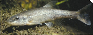
I extracted some data from the Maryland Biological Stream Survey to practice multiple regression on; the data are shown below in the SAS example. The dependent variable is the number of longnose dace (Rhinichthys cataractae) per 75-meter section of stream. The independent variables are the area (in acres) drained by the stream; the dissolved oxygen (in mg/liter); the maximum depth (in cm) of the 75-meter segment of stream; nitrate concentration (mg/liter); sulfate concentration (mg/liter); and the water temperature on the sampling date (in degrees C).
One biological goal might be to measure the physical and chemical characteristics of a stream and be able to predict the abundance of longnose dace; another goal might be to generate hypotheses about the causes of variation in longnose dace abundance.
The results of a stepwise multiple regression, with P-to-enter and P-to-leave both equal to 0.15, is that acreage, nitrate, and maximum depth contribute to the multiple regression equation. The R2 of the model including these three terms is 0.28, which isn't very high.
Graphing the results
If the multiple regression equation ends up with only two independent variables, you might be able to draw a three-dimensional graph of the relationship. Because most humans have a hard time visualizing four or more dimensions, there's no good visual way to summarize all the information in a multiple regression with three or more independent variables.
Similar tests
If the dependent variable is a nominal variable, you should do multiple logistic regression.
There are many other techniques you can use when you have three or more measurement variables, including principal components analysis, principal coordinates analysis, discriminant function analysis, hierarchical and non-hierarchical clustering, and multidimensional scaling. I'm not going to write about them; your best bet is probably to see how other researchers in your field have analyzed data similar to yours.
How to do multiple regression
Spreadsheet
If you're serious about doing multiple regressions as part of your research, you're going to have to learn a specialized statistical program such as SAS or SPSS. I've written a spreadsheet that will enable you to do a multiple regression with up to 12 X variables and up to 1000 observations. It's fun to play with, but I'm not confident enough in it that you should use it for publishable results. The spreadsheet includes histograms to help you decide whether to transform your variables, and scattergraphs of the Y variable vs. each X variable so you can see if there are any non-linear relationships. It doesn't do variable selection automatically, you manually choose which variables to include.
Web pages
I've seen a few web pages that are supposed to perform multiple regression, but I haven't been able to get them to work on my computer.
R
Salvatore Mangiafico's R Companion has a sample R program for multiple regression.
SAS
You use PROC REG to do multiple regression in SAS. Here is an example using the data on longnose dace abundance described above.
DATA fish;
   VAR stream $ longnosedace acreage do2 maxdepth no3 so4 temp;
   DATALINES;
BASIN_RUN  13  2528  9.6  80  2.28  16.75  15.3
BEAR_BR  12  3333  8.5  83  5.34  7.74  19.4
BEAR_CR  54  19611  8.3  96  0.99  10.92  19.5
BEAVER_DAM_CR  19  3570  9.2  56  5.44  16.53  17.0
BEAVER_RUN  37  1722  8.1  43  5.66  5.91  19.3
BENNETT_CR  2  583  9.2  51  2.26  8.81  12.9
BIG_BR  72  4790  9.4  91  4.10  5.65  16.7
BIG_ELK_CR  164  35971  10.2  81  3.20  17.53  13.8
BIG_PIPE_CR  18  25440  7.5  120  3.53  8.20  13.7
BLUE_LICK_RUN  1  2217  8.5  46  1.20  10.85  14.3
BROAD_RUN  53  1971  11.9  56  3.25  11.12  22.2
BUFFALO_RUN  16  12620  8.3  37  0.61  18.87  16.8
BUSH_CR  32  19046  8.3  120  2.93  11.31  18.0
CABIN_JOHN_CR  21  8612  8.2  103  1.57  16.09  15.0
CARROLL_BR  23  3896  10.4  105  2.77  12.79  18.4
COLLIER_RUN  18  6298  8.6  42  0.26  17.63  18.2
CONOWINGO_CR  112  27350  8.5  65  6.95  14.94  24.1
DEAD_RUN  25  4145  8.7  51  0.34  44.93  23.0
DEEP_RUN  5  1175  7.7  57  1.30  21.68  21.8
DEER_CR  26  8297  9.9  60  5.26  6.36  19.1
DORSEY_RUN  8  7814  6.8  160  0.44  20.24  22.6
FALLS_RUN  15  1745  9.4  48  2.19  10.27  14.3
FISHING_CR  11  5046  7.6  109  0.73  7.10  19.0
FLINTSTONE_CR  11  18943  9.2  50  0.25  14.21  18.5
GREAT_SENECA_CR  87  8624  8.6  78  3.37  7.51  21.3
GREENE_BR  33  2225  9.1  41  2.30  9.72  20.5
GUNPOWDER_FALLS  22  12659  9.7  65  3.30  5.98  18.0
HAINES_BR  98  1967  8.6  50  7.71  26.44  16.8
HAWLINGS_R  1  1172  8.3  73  2.62  4.64  20.5
HAY_MEADOW_BR  5  639  9.5  26  3.53  4.46  20.1
HERRINGTON_RUN  1  7056  6.4  60  0.25  9.82  24.5
HOLLANDS_BR  38  1934  10.5  85  2.34  11.44  12.0
ISRAEL_CR  30  6260  9.5  133  2.41  13.77  21.0
LIBERTY_RES  12  424  8.3  62  3.49  5.82  20.2
LITTLE_ANTIETAM_CR  24  3488  9.3  44  2.11  13.37  24.0
LITTLE_BEAR_CR  6  3330  9.1  67  0.81  8.16  14.9
LITTLE_CONOCOCHEAGUE_CR  15  2227  6.8  54  0.33  7.60  24.0
LITTLE_DEER_CR  38  8115  9.6  110  3.40  9.22  20.5
LITTLE_FALLS  84  1600  10.2  56  3.54  5.69  19.5
LITTLE_GUNPOWDER_R  3  15305  9.7  85  2.60  6.96  17.5
LITTLE_HUNTING_CR  18  7121  9.5  58  0.51  7.41  16.0
LITTLE_PAINT_BR  63  5794  9.4  34  1.19  12.27  17.5
MAINSTEM_PATUXENT_R  239  8636  8.4  150  3.31  5.95  18.1
MEADOW_BR  234  4803  8.5  93  5.01  10.98  24.3
MILL_CR  6  1097  8.3  53  1.71  15.77  13.1
MORGAN_RUN  76  9765  9.3  130  4.38  5.74  16.9
MUDDY_BR  25  4266  8.9  68  2.05  12.77  17.0
MUDLICK_RUN  8  1507  7.4  51  0.84  16.30  21.0
NORTH_BR  23  3836  8.3  121  1.32  7.36  18.5
NORTH_BR_CASSELMAN_R  16  17419  7.4  48  0.29  2.50  18.0
NORTHWEST_BR  6  8735  8.2  63  1.56  13.22  20.8
NORTHWEST_BR_ANACOSTIA_R  100  22550  8.4  107  1.41  14.45  23.0
OWENS_CR  80  9961  8.6  79  1.02  9.07  21.8
PATAPSCO_R  28  4706  8.9  61  4.06  9.90  19.7
PINEY_BR  48  4011  8.3  52  4.70  5.38  18.9
PINEY_CR  18  6949  9.3  100  4.57  17.84  18.6
PINEY_RUN  36  11405  9.2  70  2.17  10.17  23.6
PRETTYBOY_BR  19  904  9.8  39  6.81  9.20  19.2
RED_RUN  32  3332  8.4  73  2.09  5.50  17.7
ROCK_CR  3  575  6.8  33  2.47  7.61  18.0
SAVAGE_R  106  29708  7.7  73  0.63  12.28  21.4
SECOND_MINE_BR  62  2511  10.2  60  4.17  10.75  17.7
SENECA_CR  23  18422  9.9  45  1.58  8.37  20.1
SOUTH_BR_CASSELMAN_R  2  6311  7.6  46  0.64  21.16  18.5
SOUTH_BR_PATAPSCO  26  1450  7.9  60  2.96  8.84  18.6
SOUTH_FORK_LINGANORE_CR  20  4106  10.0  96  2.62  5.45  15.4
TUSCARORA_CR  38  10274  9.3  90  5.45  24.76  15.0
WATTS_BR   19  510  6.7  82  5.25  14.19  26.5
;
PROC REG DATA=fish;
   MODEL longnosedace=acreage do2 maxdepth no3 so4 temp /
     SELECTION=STEPWISE SLENTRY=0.15 SLSTAY=0.15 DETAILS=SUMMARY STB;
   RUN;
In the MODEL statement, the dependent variable is to the left of the equals sign, and all the independent variables are to the right. SELECTION determines which variable selection method is used; choices include FORWARD, BACKWARD, STEPWISE, and several others. You can omit the SELECTION parameter if you want to see the multiple regression model that includes all the independent variables. SLENTRY is the significance level for entering a variable into the model, or P-to-enter, if you're using FORWARD or STEPWISE selection; in this example, a variable must have a P value less than 0.15 to be entered into the regression model. SLSTAY is the significance level for removing a variable in BACKWARD or STEPWISE selection, or P-to-leave; in this example, a variable with a P value greater than 0.15 will be removed from the model. DETAILS=SUMMARY produces a shorter output file; you can omit it to see more details on each step of the variable selection process. The STB option causes the standard partial regression coefficients to be displayed.
                    Summary of Stepwise Selection

     Variable  Variable  Number   Partial    Model
Step  Entered   Removed  Vars In  R-Square R-Square   C(p)  F Value   Pr > F

 1   acreage               1       0.1201   0.1201  14.2427    9.01   0.0038
 2   no3                   2       0.1193   0.2394   5.6324   10.20   0.0022
 3   maxdepth              3       0.0404   0.2798   4.0370    3.59   0.0625
The summary shows that "acreage" was added to the model first, yielding an R2 of 0.1201. Next, "no3" was added. The R2 increased to 0.2394, and the increase in R2 was significant (P=0.0022). Next, "maxdepth" was added. The R2 increased to 0.2798, which was not quite significant (P=0.0625); SLSTAY was set to 0.15, not 0.05, because you might want to include this variable in a predictive model even if it's not quite significant. None of the other variables increased R2 enough to have a P value less than 0.15, and removing any of the variables caused a decrease in R2 big enough that P was less than 0.15, so the stepwise process is done.
                              Parameter Estimates

                Parameter     Standard                 Standardized
Variable    DF   Estimate       Error  t Value  Pr > |t|   Estimate

Intercept    1  -23.82907    15.27399   -1.56   0.1237            0
acreage      1    0.00199  0.00067421    2.95   0.0045      0.32581
maxdepth     1    0.33661     0.17757    1.90   0.0625      0.20860
no3          1    8.67304     2.77331    3.13   0.0027      0.33409
The "parameter estimates" are the partial regression coefficients; they show that the model is Ŷ=0.00199(acreage)+0.3361(maxdepth)+8.67304(no3)−23.82907. The "standardized estimates" are the standard partial regression coefficients; they show that "no3" has the greatest contribution to the model, followed by "acreage" and then "maxdepth". The value of this multiple regression would be that it suggests that the acreage of a stream's watershed is somehow important. Because watershed area wouldn't have any direct effect on the fish in the stream, I would carefully look at the correlations between the acreage and the other independent variables; I would also try to see if there are other variables that were not analyzed that might be both correlated with watershed area and directly important to fish, such as current speed, water clarity, or substrate type.
Power analysis
You need to have several times as many observations as you have independent variables, otherwise you can get "overfitting"—it could look like every independent variable is important, even if they're not. A common rule of thumb is that you should have at least 10 to 20 times as many observations as you have independent variables. You'll probably just want to collect as much data as you can afford, but if you really need to figure out how to do a formal power analysis for multiple regression, Kelley and Maxwell (2003) is a good place to start.
References
Kelley, K., and S.E. Maxwell. 2003. Sample size for multiple regression: Obtaining regression coefficients that are accurate, not simply significant. Psychological Methods 8: 305-321.
⇐ Previous topic|Next topic ⇒
Table of Contents
This page was last revised July 20, 2015. Its address is http://www.biostathandbook.com/multipleregression.html. It may be cited as:
McDonald, J.H. 2014. Handbook of Biological Statistics (3rd ed.). Sparky House Publishing, Baltimore, Maryland. This web page contains the content of pages 229-237 in the printed version.
©2014 by John H. McDonald. You can probably do what you want with this content; see the permissions page for details.