
⇐ Previous topic|Next topic ⇒
Table of Contents
Simple logistic regression
Summary
Use simple logistic regression when you have one nominal variable and one measurement variable, and you want to know whether variation in the measurement variable causes variation in the nominal variable.
When to use it
Use simple logistic regression when you have one nominal variable with two values (male/female, dead/alive, etc.) and one measurement variable. The nominal variable is the dependent variable, and the measurement variable is the independent variable.
I'm separating simple logistic regression, with only one independent variable, from multiple logistic regression, which has more than one independent variable. Many people lump all logistic regression together, but I think it's useful to treat simple logistic regression separately, because it's simpler.
Simple logistic regression is analogous to linear regression, except that the dependent variable is nominal, not a measurement. One goal is to see whether the probability of getting a particular value of the nominal variable is associated with the measurement variable; the other goal is to predict the probability of getting a particular value of the nominal variable, given the measurement variable.
| Grain size (mm) | Spiders |
|---|---|
| 0.245 | absent |
| 0.247 | absent |
| 0.285 | present |
| 0.299 | present |
| 0.327 | present |
| 0.347 | present |
| 0.356 | absent |
| 0.36 | present |
| 0.363 | absent |
| 0.364 | present |
| 0.398 | absent |
| 0.4 | present |
| 0.409 | absent |
| 0.421 | present |
| 0.432 | absent |
| 0.473 | present |
| 0.509 | present |
| 0.529 | present |
| 0.561 | absent |
| 0.569 | absent |
| 0.594 | present |
| 0.638 | present |
| 0.656 | present |
| 0.816 | present |
| 0.853 | present |
| 0.938 | present |
| 1.036 | present |
| 1.045 | present |
As an example of simple logistic regression, Suzuki et al. (2006) measured sand grain size on 28 beaches in Japan and observed the presence or absence of the burrowing wolf spider Lycosa ishikariana on each beach. Sand grain size is a measurement variable, and spider presence or absence is a nominal variable. Spider presence or absence is the dependent variable; if there is a relationship between the two variables, it would be sand grain size affecting spiders, not the presence of spiders affecting the sand.
One goal of this study would be to determine whether there was a relationship between sand grain size and the presence or absence of the species, in hopes of understanding more about the biology of the spiders. Because this species is endangered, another goal would be to find an equation that would predict the probability of a wolf spider population surviving on a beach with a particular sand grain size, to help determine which beaches to reintroduce the spider to.
You can also analyze data with one nominal and one measurement variable using a one-way anova or a Student's t–test, and the distinction can be subtle. One clue is that logistic regression allows you to predict the probability of the nominal variable. For example, imagine that you had measured the cholesterol level in the blood of a large number of 55-year-old women, then followed up ten years later to see who had had a heart attack. You could do a two-sample t–test, comparing the cholesterol levels of the women who did have heart attacks vs. those who didn't, and that would be a perfectly reasonable way to test the null hypothesis that cholesterol level is not associated with heart attacks; if the hypothesis test was all you were interested in, the t–test would probably be better than the less-familiar logistic regression. However, if you wanted to predict the probability that a 55-year-old woman with a particular cholesterol level would have a heart attack in the next ten years, so that doctors could tell their patients "If you reduce your cholesterol by 40 points, you'll reduce your risk of heart attack by X%," you would have to use logistic regression.
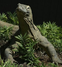
Another situation that calls for logistic regression, rather than an anova or t–test, is when you determine the values of the measurement variable, while the values of the nominal variable are free to vary. For example, let's say you are studying the effect of incubation temperature on sex determination in Komodo dragons. You raise 10 eggs at 30 °C, 30 eggs at 32°C, 12 eggs at 34°C, etc., then determine the sex of the hatchlings. It would be silly to compare the mean incubation temperatures between male and female hatchlings, and test the difference using an anova or t–test, because the incubation temperature does not depend on the sex of the offspring; you've set the incubation temperature, and if there is a relationship, it's that the sex of the offspring depends on the temperature.
When there are multiple observations of the nominal variable for each value of the measurement variable, as in the Komodo dragon example, you'll often sees the data analyzed using linear regression, with the proportions treated as a second measurement variable. Often the proportions are arc-sine transformed, because that makes the distributions of proportions more normal. This is not horrible, but it's not strictly correct. One problem is that linear regression treats all of the proportions equally, even if they are based on much different sample sizes. If 6 out of 10 Komodo dragon eggs raised at 30 °C were female, and 15 out of 30 eggs raised at 32°C were female, the 60% female at 30°C and 50% at 32°C would get equal weight in a linear regression, which is inappropriate. Logistic regression analyzes each observation (in this example, the sex of each Komodo dragon) separately, so the 30 dragons at 32°C would have 3 times the weight of the 10 dragons at 30°C.
While logistic regression with two values of the nominal variable (binary logistic regression) is by far the most common, you can also do logistic regression with more than two values of the nominal variable, called multinomial logistic regression. I'm not going to cover it here at all. Sorry.
You can also do simple logistic regression with nominal variables for both the independent and dependent variables, but to be honest, I don't understand the advantage of this over a chi-squared or G–test of independence.
Null hypothesis
The statistical null hypothesis is that the probability of a particular value of the nominal variable is not associated with the value of the measurement variable; in other words, the line describing the relationship between the measurement variable and the probability of the nominal variable has a slope of zero.
How the test works
Simple logistic regression finds the equation that best predicts the value of the Y variable for each value of the X variable. What makes logistic regression different from linear regression is that you do not measure the Y variable directly; it is instead the probability of obtaining a particular value of a nominal variable. For the spider example, the values of the nominal variable are "spiders present" and "spiders absent." The Y variable used in logistic regression would then be the probability of spiders being present on a beach. This probability could take values from 0 to 1. The limited range of this probability would present problems if used directly in a regression, so the odds, Y/(1-Y), is used instead. (If the probability of spiders on a beach is 0.25, the odds of having spiders are 0.25/(1-0.25)=1/3. In gambling terms, this would be expressed as "3 to 1 odds against having spiders on a beach.") Taking the natural log of the odds makes the variable more suitable for a regression, so the result of a logistic regression is an equation that looks like this:
ln[Y/(1−Y)]=a+bX
You find the slope (b) and intercept (a) of the best-fitting equation in a logistic regression using the maximum-likelihood method, rather than the least-squares method you use for linear regression. Maximum likelihood is a computer-intensive technique; the basic idea is that it finds the values of the parameters under which you would be most likely to get the observed results.
For the spider example, the equation is
ln[Y/(1−Y)]=−1.6476+5.1215(grain size)
Rearranging to solve for Y (the probability of spiders on a beach) yields
Y=e−1.6476+5.1215(grain size)/(1+e−1.6476+5.1215(grain size))
where e is the root of natural logs. So if you went to a beach and wanted to predict the probability that spiders would live there, you could measure the sand grain size, plug it into the equation, and get an estimate of Y, the probability of spiders being on the beach.
There are several different ways of estimating the P value. The Wald chi-square is fairly popular, but it may yield inaccurate results with small sample sizes. The likelihood ratio method may be better. It uses the difference between the probability of obtaining the observed results under the logistic model and the probability of obtaining the observed results in a model with no relationship between the independent and dependent variables. I recommend you use the likelihood-ratio method; be sure to specify which method you've used when you report your results.
For the spider example, the P value using the likelihood ratio method is 0.033, so you would reject the null hypothesis. The P value for the Wald method is 0.088, which is not quite significant.
Assumptions
Simple logistic regression assumes that the observations are independent; in other words, that one observation does not affect another. In the Komodo dragon example, if all the eggs at 30°C were laid by one mother, and all the eggs at 32°C were laid by a different mother, that would make the observations non-independent. If you design your experiment well, you won't have a problem with this assumption.
Simple logistic regression assumes that the relationship between the natural log of the odds ratio and the measurement variable is linear. You might be able to fix this with a transformation of your measurement variable, but if the relationship looks like a U or upside-down U, a transformation won't work. For example, Suzuki et al. (2006) found an increasing probability of spiders with increasing grain size, but I'm sure that if they looked at beaches with even larger sand (in other words, gravel), the probability of spiders would go back down. In that case you couldn't do simple logistic regression; you'd probably want to do multiple logistic regression with an equation including both X and X2 terms, instead.
Simple logistic regression does not assume that the measurement variable is normally distributed.
Examples
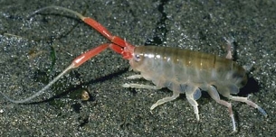
McDonald (1985) counted allele frequencies at the mannose-6-phosphate isomerase (Mpi) locus in the amphipod crustacean Megalorchestia californiana, which lives on sandy beaches of the Pacific coast of North America. There were two common alleles, Mpi90 and Mpi100. The latitude of each collection location, the count of each of the alleles, and the proportion of the Mpi100 allele, are shown here:
| Location | Latitude | Mpi90 | Mpi100 | p, Mpi100 |
|---|---|---|---|---|
| Port Townsend, WA | 48.1 | 47 | 139 | 0.748 |
| Neskowin, OR | 45.2 | 177 | 241 | 0.577 |
| Siuslaw R., OR | 44 | 1087 | 1183 | 0.521 |
| Umpqua R., OR | 43.7 | 187 | 175 | 0.483 |
| Coos Bay, OR | 43.5 | 397 | 671 | 0.628 |
| San Francisco, CA | 37.8 | 40 | 14 | 0.259 |
| Carmel, CA | 36.6 | 39 | 17 | 0.304 |
| Santa Barbara, CA | 34.3 | 30 | 0 | 0 |
Allele (Mpi90 or Mpi100) is the nominal variable, and latitude is the measurement variable. If the biological question were "Do different locations have different allele frequencies?", you would ignore latitude and do a chi-square or G–test of independence; here the biological question is "Are allele frequencies associated with latitude?"
Note that although the proportion of the Mpi100 allele seems to increase with increasing latitude, the sample sizes for the northern and southern areas are pretty small; doing a linear regression of allele frequency vs. latitude would give them equal weight to the much larger samples from Oregon, which would be inappropriate. Doing a logistic regression, the result is chi2=83.3, 1 d.f., P=7×10⁻²⁰. The equation of the relationship is
ln(Y/(1−Y))=−7.6469+0.1786(latitude),
where Y is the predicted probability of getting an Mpi100 allele. Solving this for Y gives
Y=e−7.6469+0.1786(latitude)/(1+e−7.6469+0.1786(latitude)).
This logistic regression line is shown on the graph; note that it has a gentle S-shape. All logistic regression equations have an S-shape, although it may not be obvious if you look over a narrow range of values.
 Mpi allele frequencies vs. latitude in the amphipod Megalorchestia californiana. Error bars are 95% confidence intervals; the thick black line is the logistic regression line.
Graphing the results
If you have multiple observations for each value of the measurement variable, as in the amphipod example above, you can plot a scattergraph with the measurement variable on the X axis and the proportions on the Y axis. You might want to put 95% confidence intervals on the points; this gives a visual indication of which points contribute more to the regression (the ones with larger sample sizes have smaller confidence intervals).
There's no automatic way in spreadsheets to add the logistic regression line. Here's how I got it onto the graph of the amphipod data. First, I put the latitudes in column A and the proportions in column B. Then, using the Fill: Series command, I added numbers 30, 30.1, 30.2,…50 to cells A10 through A210. In column C I entered the equation for the logistic regression line; in Excel format, it's
=exp(-7.6469+0.1786*(A10))/(1+exp(-7.6469+0.1786*(A10)))
for row 10. I copied this into cells C11 through C210. Then when I drew a graph of the numbers in columns A, B, and C, I gave the numbers in column B symbols but no line, and the numbers in column C got a line but no symbols.
If you only have one observation of the nominal variable for each value of the measurement variable, as in the spider example, it would be silly to draw a scattergraph, as each point on the graph would be at either 0 or 1 on the Y axis. If you have lots of data points, you can divide the measurement values into intervals and plot the proportion for each interval on a bar graph. Here is data from the Maryland Biological Stream Survey on 2180 sampling sites in Maryland streams. The measurement variable is dissolved oxygen concentration, and the nominal variable is the presence or absence of the central stoneroller, Campostoma anomalum. If you use a bar graph to illustrate a logistic regression, you should explain that the grouping was for heuristic purposes only, and the logistic regression was done on the raw, ungrouped data.

Similar tests
You can do logistic regression with a dependent variable that has more than two values, known as multinomial, polytomous, or polychotomous logistic regression. I don't cover this here.
Use multiple logistic regression when the dependent variable is nominal and there is more than one independent variable. It is analogous to multiple linear regression, and all of the same caveats apply.
Use linear regression when the Y variable is a measurement variable.
When there is just one measurement variable and one nominal variable, you could use one-way anova or a t–test to compare the means of the measurement variable between the two groups. Conceptually, the difference is whether you think variation in the nominal variable causes variation in the measurement variable (use a t–test) or variation in the measurement variable causes variation in the probability of the nominal variable (use logistic regression). You should also consider who you are presenting your results to, and how they are going to use the information. For example, Tallamy et al. (2003) examined mating behavior in spotted cucumber beetles (Diabrotica undecimpunctata). Male beetles stroke the female with their antenna, and Tallamy et al. wanted to know whether faster-stroking males had better mating success. They compared the mean stroking rate of 21 successful males (50.9 strokes per minute) and 16 unsuccessful males (33.8 strokes per minute) with a two-sample t–test, and found a significant result (P<0.0001). This is a simple and clear result, and it answers the question, "Are female spotted cucumber beetles more likely to mate with males who stroke faster?" Tallamy et al. (2003) could have analyzed these data using logistic regression; it is a more difficult and less familiar statistical technique that might confuse some of their readers, but in addition to answering the yes/no question about whether stroking speed is related to mating success, they could have used the logistic regression to predict how much increase in mating success a beetle would get as it increased its stroking speed. This could be useful additional information (especially if you're a male cucumber beetle).
How to do the test
Spreadsheet
I have written a spreadsheet to do simple logistic regression. You can enter the data either in summarized form (for example, saying that at 30°C there were 7 male and 3 female Komodo dragons) or non-summarized form (for example, entering each Komodo dragon separately, with "0" for a male and "1" for a female). It uses the likelihood-ratio method for calculating the P value. The spreadsheet makes use of the "Solver" tool in Excel. If you don't see Solver listed in the Tools menu, go to Add-Ins in the Tools menu and install Solver.
The spreadsheet is fun to play with, but I'm not confident enough in it to recommend that you use it for publishable results.
Web page
There is a very nice web page that will do logistic regression, with the likelihood-ratio chi-square. You can enter the data either in summarized form or non-summarized form, with the values separated by tabs (which you'll get if you copy and paste from a spreadsheet) or commas. You would enter the amphipod data like this:
 48.1,47,139
 45.2,177,241
 44.0,1087,1183
 43.7,187,175
 43.5,397,671
 37.8,40,14
 36.6,39,17
 34.3,30,0
R
Salvatore Mangiafico's R Companion has a sample R program for simple logistic regression.
SAS
Use PROC LOGISTIC for simple logistic regression. There are two forms of the MODEL statement. When you have multiple observations for each value of the measurement variable, your data set can have the measurement variable, the number of "successes" (this can be either value of the nominal variable), and the total (which you may need to create a new variable for, as shown here). Here is an example using the amphipod data:
DATA amphipods;
   INPUT location $ latitude mpi90 mpi100;
   total=mpi90+mpi100;
   DATALINES;
Port_Townsend,_WA    48.1      47    139
Neskowin,_OR         45.2     177    241
Siuslaw_R.,_OR       44.0    1087   1183
Umpqua_R.,_OR        43.7     187    175
Coos_Bay,_OR         43.5     397    671
San_Francisco,_CA    37.8      40     14
Carmel,_CA           36.6      39     17
Santa_Barbara,_CA    34.3      30      0
;
PROC LOGISTIC DATA=amphipods;
   MODEL mpi100/total=latitude;
RUN;
Note that you create the new variable TOTAL in the DATA step by adding the number of Mpi90 and Mpi100 alleles. The MODEL statement uses the number of Mpi100 alleles out of the total as the dependent variable. The P value would be the same if you used Mpi90; the equation parameters would be different.
There is a lot of output from PROC LOGISTIC that you don't need. The program gives you three different P values; the likelihood ratio P value is the most commonly used:
     Testing Global Null Hypothesis: BETA=0

Test               Chi-Square     DF   Pr > ChiSq

Likelihood Ratio      83.3007      1       <.0001 P value
Score                 80.5733      1       <.0001
Wald                  72.0755      1       <.0001
The coefficients of the logistic equation are given under "estimate":
              Analysis of Maximum Likelihood Estimates

                            Standard         Wald
Parameter   DF   Estimate      Error   Chi-Square   Pr > ChiSq

Intercept    1    -7.6469     0.9249      68.3605       <.0001
latitude     1     0.1786     0.0210      72.0755       <.0001
Using these coefficients, the maximum likelihood equation for the proportion of Mpi100 alleles at a particular latitude is
Y=e−7.6469+0.1786(latitude)/(1+e−7.6469+0.1786(latitude))
It is also possible to use data in which each line is a single observation. In that case, you may use either words or numbers for the dependent variable. In this example, the data are height (in inches) of the 2004 students of my class, along with their favorite insect (grouped into beetles vs. everything else, where "everything else" includes spiders, which a biologist really should know are not insects):
DATA insect;
   INPUT height insect $ @@;
   DATALINES;
62  beetle  66  other  61  beetle  67  other   62  other
76  other   66  other  70  beetle  67  other   66  other
70  other   70  other  77  beetle  76  other   72  beetle
76  beetle  72  other  70  other   65  other   63  other
63  other   70  other  72  other   70  beetle  74  other
;
PROC LOGISTIC DATA=insect;
   MODEL insect=height;
RUN;
The format of the results is the same for either form of the MODEL statement. In this case, the model would be the probability of BEETLE, because it is alphabetically first; to model the probability of OTHER, you would add an EVENT after the nominal variable in the MODEL statement, making it "MODEL insect (EVENT='other')=height;"
Power analysis
You can use G*Power to estimate the sample size needed for a simple logistic regression. Choose "z tests" under Test family and "Logistic regression" under Statistical test. Set the number of tails (usually two), alpha (usually 0.05), and power (often 0.8 or 0.9). For simple logistic regression, set "X distribution" to Normal, "R2 other X" to 0, "X parm μ" to 0, and "X parm σ" to 1.
The last thing to set is your effect size. This is the odds ratio of the difference you're hoping to find between the odds of Y when X is equal to the mean X, and the odds of Y when X is equal to the mean X plus one standard deviation. You can click on the "Determine" button to calculate this.
For example, let's say you want to study the relationship between sand particle size and the presences or absence of tiger beetles. You set alpha to 0.05 and power to 0.90. You expect, based on previous research, that 30% of the beaches you'll look at will have tiger beetles, so you set "Pr(Y=1|X=1) H0" to 0.30. Also based on previous research, you expect a mean sand grain size of .6 mm with a standard deviation of 0.2 mm. The effect size (the minimum deviation from the null hypothesis that you hope to see) is that as the sand grain size increases by one standard deviation, from 0.6 mm to 0.8 mm, the proportion of beaches with tiger beetles will go from 0.30 to 0.40. You click on the "Determine" button and enter 0.40 for "Pr(Y=1|X=1) H1" and 0.30 for "Pr(Y=1|X=1) H0", then hit "Calculate and transfer to main window." It will fill in the odds ratio (1.555 for our example) and the "Pr(Y=1|X=1) H0". The result in this case is 206, meaning your experiment is going to require that you travel to 206 warm, beautiful beaches.
References
McDonald, J.H. 1985. Size-related and geographic variation at two enzyme loci in Megalorchestia californiana (Amphipoda: Talitridae). Heredity 54: 359-366.
Suzuki, S., N. Tsurusaki, and Y. Kodama. 2006. Distribution of an endangered burrowing spider Lycosa ishikariana in the San'in Coast of Honshu, Japan (Araneae: Lycosidae). Acta Arachnologica 55: 79-86.
Tallamy, D.W., M.B. Darlington, J.D. Pesek, and B.E. Powell. 2003. Copulatory courtship signals male genetic quality in cucumber beetles. Proceedings of the Royal Society of London B 270: 77-82.
⇐ Previous topic|Next topic ⇒
Table of Contents
This page was last revised July 20, 2015. Its address is http://www.biostathandbook.com/logistic.html. It may be cited as:
McDonald, J.H. 2014. Handbook of Biological Statistics (3rd ed.). Sparky House Publishing, Baltimore, Maryland. This web page contains the content of pages 238-246 in the printed version.
©2014 by John H. McDonald. You can probably do what you want with this content; see the permissions page for details.