Search the handbook:

⇐ Previous topic|Next topic ⇒
Table of Contents

---

One-way anova

---

Summary

Use one-way anova when you have one nominal variable and one measurement variable; the nominal variable divides the measurements into two or more groups. It tests whether the means of the measurement variable are the same for the different groups.

When to use it

Analysis of variance (anova) is the most commonly used technique for comparing the means of groups of measurement data. There are lots of different experimental designs that can be analyzed with different kinds of anova; in this handbook, I describe only one-way anova, nested anova and two-way anova.

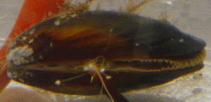
In a one-way anova (also known as a one-factor, single-factor, or single-classification anova), there is one measurement variable and one nominal variable. You make multiple observations of the measurement variable for each value of the nominal variable. For example, here are some data on a shell measurement (the length of the anterior adductor muscle scar, standardized by dividing by length; I'll call this "AAM length") in the mussel Mytilus trossulus from five locations: Tillamook, Oregon; Newport, Oregon; Petersburg, Alaska; Magadan, Russia; and Tvarminne, Finland, taken from a much larger data set used in McDonald et al. (1991).

Tillamook	Newport	Petersburg	Magadan	Tvarminne
0.0571	0.0873	0.0974	0.1033	0.0703
0.0813	0.0662	0.1352	0.0915	0.1026
0.0831	0.0672	0.0817	0.0781	0.0956
0.0976	0.0819	0.1016	0.0685	0.0973
0.0817	0.0749	0.0968	0.0677	0.1039
0.0859	0.0649	0.1064	0.0697	0.1045
0.0735	0.0835	0.105	0.0764
0.0659	0.0725		0.0689
0.0923
0.0836

The nominal variable is location, with the five values Tillamook, Newport, Petersburg, Magadan, and Tvarminne. There are six to ten observations of the measurement variable, AAM length, from each location.

Null hypothesis

The statistical null hypothesis is that the means of the measurement variable are the same for the different categories of data; the alternative hypothesis is that they are not all the same. For the example data set, the null hypothesis is that the mean AAM length is the same at each location, and the alternative hypothesis is that the mean AAM lengths are not all the same.

How the test works

The basic idea is to calculate the mean of the observations within each group, then compare the variance among these means to the average variance within each group. Under the null hypothesis that the observations in the different groups all have the same mean, the weighted among-group variance will be the same as the within-group variance. As the means get further apart, the variance among the means increases. The test statistic is thus the ratio of the variance among means divided by the average variance within groups, or F_s. This statistic has a known distribution under the null hypothesis, so the probability of obtaining the observed F_s under the null hypothesis can be calculated.

The shape of the F-distribution depends on two degrees of freedom, the degrees of freedom of the numerator (among-group variance) and degrees of freedom of the denominator (within-group variance). The among-group degrees of freedom is the number of groups minus one. The within-groups degrees of freedom is the total number of observations, minus the number of groups. Thus if there are n observations in a groups, numerator degrees of freedom is a-1 and denominator degrees of freedom is n-a. For the example data set, there are 5 groups and 39 observations, so the numerator degrees of freedom is 4 and the denominator degrees of freedom is 34. Whatever program you use for the anova will almost certainly calculate the degrees of freedom for you.

The conventional way of reporting the complete results of an anova is with a table (the "sum of squares" column is often omitted). Here are the results of a one-way anova on the mussel data:

	sum of squares	d.f.	mean square	Fs	P
among groups	0.00452	4	0.001113	7.12	2.8×10-4
within groups	0.00539	34	0.000159
total	0.00991	38

If you're not going to use the mean squares for anything, you could just report this as "The means were significantly heterogeneous (one-way anova, F_{4, 34}=7.12, P=2.8×10^-4)." The degrees of freedom are given as a subscript to F, with the numerator first.

Note that statisticians often call the within-group mean square the "error" mean square. I think this can be confusing to non-statisticians, as it implies that the variation is due to experimental error or measurement error. In biology, the within-group variation is often largely the result of real, biological variation among individuals, not the kind of mistakes implied by the word "error." That's why I prefer the term "within-group mean square."

Assumptions

One-way anova assumes that the observations within each group are normally distributed. It is not particularly sensitive to deviations from this assumption; if you apply one-way anova to data that are non-normal, your chance of getting a P value less than 0.05, if the null hypothesis is true, is still pretty close to 0.05. It's better if your data are close to normal, so after you collect your data, you should calculate the residuals (the difference between each observation and the mean of its group) and plot them on a histogram. If the residuals look severely non-normal, try data transformations and see if one makes the data look more normal.

If none of the transformations you try make the data look normal enough, you can use the Kruskal-Wallis test. Be aware that it makes the assumption that the different groups have the same shape of distribution, and that it doesn't test the same null hypothesis as one-way anova. Personally, I don't like the Kruskal-Wallis test; I recommend that if you have non-normal data that can't be fixed by transformation, you go ahead and use one-way anova, but be cautious about rejecting the null hypothesis if the P value is not very far below 0.05 and your data are extremely non-normal.

One-way anova also assumes that your data are homoscedastic, meaning the standard deviations are equal in the groups. You should examine the standard deviations in the different groups and see if there are big differences among them.

If you have a balanced design, meaning that the number of observations is the same in each group, then one-way anova is not very sensitive to heteroscedasticity (different standard deviations in the different groups). I haven't found a thorough study of the effects of heteroscedasticity that considered all combinations of the number of groups, sample size per group, and amount of heteroscedasticity. I've done simulations with two groups, and they indicated that heteroscedasticity will give an excess proportion of false positives for a balanced design only if one standard deviation is at least three times the size of the other, and the sample size in each group is fewer than 10. I would guess that a similar rule would apply to one-way anovas with more than two groups and balanced designs.

Heteroscedasticity is a much bigger problem when you have an unbalanced design (unequal sample sizes in the groups). If the groups with smaller sample sizes also have larger standard deviations, you will get too many false positives. The difference in standard deviations does not have to be large; a smaller group could have a standard deviation that's 50% larger, and your rate of false positives could be above 10% instead of at 5% where it belongs. If the groups with larger sample sizes have larger standard deviations, the error is in the opposite direction; you get too few false positives, which might seem like a good thing except it also means you lose power (get too many false negatives, if there is a difference in means).

You should try really hard to have equal sample sizes in all of your groups. With a balanced design, you can safely use a one-way anova unless the sample sizes per group are less than 10 and the standard deviations vary by threefold or more. If you have a balanced design with small sample sizes and very large variation in the standard deviations, you should use Welch's anova instead.

If you have an unbalanced design, you should carefully examine the standard deviations. Unless the standard deviations are very similar, you should probably use Welch's anova. It is less powerful than one-way anova for homoscedastic data, but it can be much more accurate for heteroscedastic data from an unbalanced design.

Additional analyses

Tukey-Kramer test

If you reject the null hypothesis that all the means are equal, you'll probably want to look at the data in more detail. One common way to do this is to compare different pairs of means and see which are significantly different from each other. For the mussel shell example, the overall P value is highly significant; you would probably want to follow up by asking whether the mean in Tillamook is different from the mean in Newport, whether Newport is different from Petersburg, etc.

It might be tempting to use a simple two-sample t–test on each pairwise comparison that looks interesting to you. However, this can result in a lot of false positives. When there are a groups, there are (a²−a)/2 possible pairwise comparisons, a number that quickly goes up as the number of groups increases. With 5 groups, there are 10 pairwise comparisons; with 10 groups, there are 45, and with 20 groups, there are 190 pairs. When you do multiple comparisons, you increase the probability that at least one will have a P value less than 0.05 purely by chance, even if the null hypothesis of each comparison is true.

There are a number of different tests for pairwise comparisons after a one-way anova, and each has advantages and disadvantages. The differences among their results are fairly subtle, so I will describe only one, the Tukey-Kramer test. It is probably the most commonly used post-hoc test after a one-way anova, and it is fairly easy to understand.

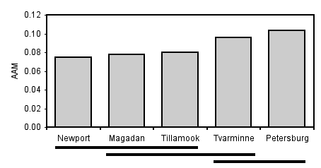
In the Tukey–Kramer method, the minimum significant difference (MSD) is calculated for each pair of means. It depends on the sample size in each group, the average variation within the groups, and the total number of groups. For a balanced design, all of the MSDs will be the same; for an unbalanced design, pairs of groups with smaller sample sizes will have bigger MSDs. If the observed difference between a pair of means is greater than the MSD, the pair of means is significantly different. For example, the Tukey MSD for the difference between Newport and Tillamook is 0.0172. The observed difference between these means is 0.0054, so the difference is not significant. Newport and Petersburg have a Tukey MSD of 0.0188; the observed difference is 0.0286, so it is significant.

There are a couple of common ways to display the results of the Tukey–Kramer test. One technique is to find all the sets of groups whose means do not differ significantly from each other, then indicate each set with a different symbol.

Location	mean AAM	Tukey–Kramer
Newport	0.0748	a
Magadan	0.0780	a, b
Tillamook	0.0802	a, b
Tvarminne	0.0957	b, c
Petersburg	0.103	c

Then you explain that "Means with the same letter are not significantly different from each other (Tukey–Kramer test, P>0.05)." This table shows that Newport and Magadan both have an "a", so they are not significantly different; Newport and Tvarminne don't have the same letter, so they are significantly different.

Another way you can illustrate the results of the Tukey–Kramer test is with lines connecting means that are not significantly different from each other. This is easiest when the means are sorted from smallest to largest:

There are also tests to compare different sets of groups; for example, you could compare the two Oregon samples (Newport and Tillamook) to the two samples from further north in the Pacific (Magadan and Petersburg). The Scheffé test is probably the most common. The problem with these tests is that with a moderate number of groups, the number of possible comparisons becomes so large that the P values required for significance become ridiculously small.

Partitioning variance

The most familiar one-way anovas are "fixed effect" or "model I" anovas. The different groups are interesting, and you want to know which are different from each other. As an example, you might compare the AAM length of the mussel species Mytilus edulis, Mytilus galloprovincialis, Mytilus trossulus and Mytilus californianus; you'd want to know which had the longest AAM, which was shortest, whether M. edulis was significantly different from M. trossulus, etc.

The other kind of one-way anova is a "random effect" or "model II" anova. The different groups are random samples from a larger set of groups, and you're not interested in which groups are different from each other. An example would be taking offspring from five random families of M. trossulus and comparing the AAM lengths among the families. You wouldn't care which family had the longest AAM, and whether family A was significantly different from family B; they're just random families sampled from a much larger possible number of families. Instead, you'd be interested in how the variation among families compared to the variation within families; in other words, you'd want to partition the variance.

Under the null hypothesis of homogeneity of means, the among-group mean square and within-group mean square are both estimates of the within-group parametric variance. If the means are heterogeneous, the within-group mean square is still an estimate of the within-group variance, but the among-group mean square estimates the sum of the within-group variance plus the group sample size times the added variance among groups. Therefore subtracting the within-group mean square from the among-group mean square, and dividing this difference by the average group sample size, gives an estimate of the added variance component among groups. The equation is:

among-group variance=(MS_among−MS_within)/n_o

where n_o is a number that is close to, but usually slightly less than, the arithmetic mean of the sample size (n_i) of each of the a groups:

n_o=(1/(a−1))*(sum(n_i)−(sum(n_i²)/sum(n_i)).

Each component of the variance is often expressed as a percentage of the total variance components. Thus an anova table for a one-way anova would indicate the among-group variance component and the within-group variance component, and these numbers would add to 100%.

Although statisticians say that each level of an anova "explains" a proportion of the variation, this statistical jargon does not mean that you've found a biological cause-and-effect explanation. If you measure the number of ears of corn per stalk in 10 random locations in a field, analyze the data with a one-way anova, and say that the location "explains" 74.3% of the variation, you haven't really explained anything; you don't know whether some areas have higher yield because of different water content in the soil, different amounts of insect damage, different amounts of nutrients in the soil, or random attacks by a band of marauding corn bandits.

Partitioning the variance components is particularly useful in quantitative genetics, where the within-family component might reflect environmental variation while the among-family component reflects genetic variation. Of course, estimating heritability involves more than just doing a simple anova, but the basic concept is similar.

Another area where partitioning variance components is useful is in designing experiments. For example, let's say you're planning a big experiment to test the effect of different drugs on calcium uptake in rat kidney cells. You want to know how many rats to use, and how many measurements to make on each rat, so you do a pilot experiment in which you measure calcium uptake on 6 rats, with 4 measurements per rat. You analyze the data with a one-way anova and look at the variance components. If a high percentage of the variation is among rats, that would tell you that there's a lot of variation from one rat to the next, but the measurements within one rat are pretty uniform. You could then design your big experiment to include a lot of rats for each drug treatment, but not very many measurements on each rat. Or you could do some more pilot experiments to try to figure out why there's so much rat-to-rat variation (maybe the rats are different ages, or some have eaten more recently than others, or some have exercised more) and try to control it. On the other hand, if the among-rat portion of the variance was low, that would tell you that the mean values for different rats were all about the same, while there was a lot of variation among the measurements on each rat. You could design your big experiment with fewer rats and more observations per rat, or you could try to figure out why there's so much variation among measurements and control it better.

There's an equation you can use for optimal allocation of resources in experiments. It's usually used for nested anova, but you can use it for a one-way anova if the groups are random effect (model II).

Partitioning the variance applies only to a model II (random effects) one-way anova. It doesn't really tell you anything useful about the more common model I (fixed effects) one-way anova, although sometimes people like to report it (because they're proud of how much of the variance their groups "explain," I guess).

Example

Here are data on the genome size (measured in picograms of DNA per haploid cell) in several large groups of crustaceans, taken from Gregory (2014). The cause of variation in genome size has been a puzzle for a long time; I'll use these data to answer the biological question of whether some groups of crustaceans have different genome sizes than others. Because the data from closely related species would not be independent (closely related species are likely to have similar genome sizes, because they recently descended from a common ancestor), I used a random number generator to randomly choose one species from each family.

Amphipods	Barnacles	Branchiopods	Copepods	Decapods	Isopods	Ostracods
0.74	0.67	0.19	0.25	1.60	1.71	0.46
0.95	0.90	0.21	0.25	1.65	2.35	0.70
1.71	1.23	0.22	0.58	1.80	2.40	0.87
1.89	1.40	0.22	0.97	1.90	3.00	1.47
3.80	1.46	0.28	1.63	1.94	5.65	3.13
3.97	2.60	0.30	1.77	2.28	5.70
7.16		0.40	2.67	2.44	6.79
8.48		0.47	5.45	2.66	8.60
13.49		0.63	6.81	2.78	8.82
16.09		0.87		2.80
27.00		2.77		2.83
50.91		2.91		3.01
64.62				4.34
				4.50
				4.55
				4.66
				4.70
				4.75
				4.84
				5.23
				6.20
				8.29
				8.53
				10.58
				15.56
				22.16
				38.00
				38.47
				40.89

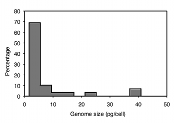
After collecting the data, the next step is to see if they are normal and homoscedastic. It's pretty obviously non-normal; most of the values are less than 10, but there are a small number that are much higher. A histogram of the largest group, the decapods (crabs, shrimp and lobsters), makes this clear:

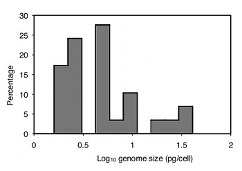
The data are also highly heteroscedastic; the standard deviations range from 0.67 in barnacles to 20.4 in amphipods. Fortunately, log-transforming the data make them closer to homoscedastic (standard deviations ranging from 0.20 to 0.63) and look more normal:

Analyzing the log-transformed data with one-way anova, the result is F_6,76=11.72, P=2.9×10⁻⁹. So there is very significant variation in mean genome size among these seven taxonomic groups of crustaceans.

The next step is to use the Tukey-Kramer test to see which pairs of taxa are significantly different in mean genome size. The usual way to display this information is by identifying groups that are not significantly different; here I do this with horizontal bars:

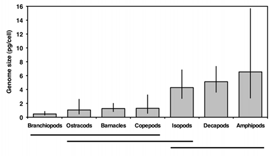
This graph suggests that there are two sets of genome sizes, groups with small genomes (branchiopods, ostracods, barnacles, and copepods) and groups with large genomes (decapods and amphipods); the members of each set are not significantly different from each other. Isopods are in the middle; the only group they're significantly different from is branchiopods. So the answer to the original biological question, "do some groups of crustaceans have different genome sizes than others," is yes. Why different groups have different genome sizes remains a mystery.

Graphing the results

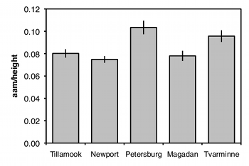
The usual way to graph the results of a one-way anova is with a bar graph. The heights of the bars indicate the means, and there's usually some kind of error bar, either 95% confidence intervals or standard errors. Be sure to say in the figure caption what the error bars represent.

Similar tests

If you have only two groups, you can do a two-sample t–test. This is mathematically equivalent to an anova and will yield the exact same P value, so if all you'll ever do is comparisons of two groups, you might as well call them t–tests. If you're going to do some comparisons of two groups, and some with more than two groups, it will probably be less confusing if you call all of your tests one-way anovas.

If there are two or more nominal variables, you should use a two-way anova, a nested anova, or something more complicated that I won't cover here. If you're tempted to do a very complicated anova, you may want to break your experiment down into a set of simpler experiments for the sake of comprehensibility.

If the data severely violate the assumptions of the anova, you can use Welch's anova if the standard deviations are heterogeneous or use the Kruskal-Wallis test if the distributions are non-normal.

How to do the test

Spreadsheet

I have put together a spreadsheet to do one-way anova on up to 50 groups and 1000 observations per group. It calculates the P value, does the Tukey–Kramer test, and partitions the variance.

Some versions of Excel include an "Analysis Toolpak," which includes an "Anova: Single Factor" function that will do a one-way anova. You can use it if you want, but I can't help you with it. It does not include any techniques for unplanned comparisons of means, and it does not partition the variance.

Web pages

Several people have put together web pages that will perform a one-way anova; one good one is here. It is easy to use, and will handle three to 26 groups and 3 to 1024 observations per group. It does not do the Tukey-Kramer test and does not partition the variance.

R

Salvatore Mangiafico's R Companion has a sample R program for one-way anova.

SAS

There are several SAS procedures that will perform a one-way anova. The two most commonly used are PROC ANOVA and PROC GLM. Either would be fine for a one-way anova, but PROC GLM (which stands for "General Linear Models") can be used for a much greater variety of more complicated analyses, so you might as well use it for everything.

Here is a SAS program to do a one-way anova on the mussel data from above.

DATA musselshells;
   INPUT location $ aam @@;
   DATALINES;
Tillamook  0.0571  Tillamook  0.0813  Tillamook  0.0831  Tillamook  0.0976  
Tillamook  0.0817  Tillamook  0.0859  Tillamook  0.0735  Tillamook  0.0659  
Tillamook  0.0923  Tillamook  0.0836  
Newport    0.0873  Newport    0.0662  Newport    0.0672  Newport    0.0819  
Newport    0.0749  Newport    0.0649  Newport    0.0835  Newport    0.0725  
Petersburg 0.0974  Petersburg 0.1352  Petersburg 0.0817  Petersburg 0.1016  
Petersburg 0.0968  Petersburg 0.1064  Petersburg 0.1050  
Magadan    0.1033  Magadan    0.0915  Magadan    0.0781  Magadan    0.0685  
Magadan    0.0677  Magadan    0.0697  Magadan    0.0764  Magadan    0.0689  
Tvarminne  0.0703  Tvarminne  0.1026  Tvarminne  0.0956  Tvarminne  0.0973  
Tvarminne  0.1039  Tvarminne  0.1045
;
PROC glm DATA=musselshells;
  CLASS location;
  MODEL aam = location;
RUN;

The output includes the traditional anova table; the P value is given under "Pr > F".

                            Sum of
Source            DF       Squares    Mean Square   F Value   Pr > F

Model              4    0.00451967     0.00112992     7.12    0.0003
Error             34    0.00539491     0.00015867                     
Corrected Total   38    0.00991458

PROC GLM doesn't calculate the variance components for an anova. Instead, you use PROC VARCOMP. You set it up just like PROC GLM, with the addition of METHOD=TYPE1 (where "TYPE1" includes the numeral 1, not the letter el. The procedure has four different methods for estimating the variance components, and TYPE1 seems to be the same technique as the one I've described above. Here's how to do the one-way anova, including estimating the variance components, for the mussel shell example.

PROC GLM DATA=musselshells;
  CLASS location;
  MODEL aam = location;
PROC VARCOMP DATA=musselshells METHOD=TYPE1;
  CLASS location;
  MODEL aam = location;
RUN;

The results include the following:

       Type 1 Estimates
 
Variance Component        Estimate

Var(location)            0.0001254
Var(Error)               0.0001587

The output is not given as a percentage of the total, so you'll have to calculate that. For these results, the among-group component is 0.0001254/(0.0001254+0.0001586)=0.4415, or 44.15%; the within-group component is 0.0001587/(0.0001254+0.0001586)=0.5585, or 55.85%.

Welch's anova

If the data show a lot of heteroscedasticity (different groups have different standard deviations), the one-way anova can yield an inaccurate P value; the probability of a false positive may be much higher than 5%. In that case, you should use Welch's anova. I've written a spreadsheet to do Welch's anova. It includes the Games-Howell test, which is similar to the Tukey-Kramer test for a regular anova. (Note: the original spreadsheet gave incorrect results for the Games-Howell test; it was corrected on April 28, 2015). You can do Welch's anova in SAS by adding a MEANS statement, the name of the nominal variable, and the word WELCH following a slash. Unfortunately, SAS does not do the Games-Howell post-hoc test. Here is the example SAS program from above, modified to do Welch's anova:

PROC GLM DATA=musselshells;
  CLASS location;
  MODEL aam = location;
  MEANS location / WELCH;
RUN;

Here is part of the output:

            Welch's ANOVA for aam
 
 Source            DF    F Value    Pr > F

 location      4.0000       5.66    0.0051
 Error        15.6955 

Power analysis

To do a power analysis for a one-way anova is kind of tricky, because you need to decide what kind of effect size you're looking for. If you're mainly interested in the overall significance test, the sample size needed is a function of the standard deviation of the group means. Your estimate of the standard deviation of means that you're looking for may be based on a pilot experiment or published literature on similar experiments.

If you're mainly interested in the comparisons of means, there are other ways of expressing the effect size. Your effect could be a difference between the smallest and largest means, for example, that you would want to be significant by a Tukey-Kramer test. There are ways of doing a power analysis with this kind of effect size, but I don't know much about them and won't go over them here.

To do a power analysis for a one-way anova using the free program G*Power, choose "F tests" from the "Test family" menu and "ANOVA: Fixed effects, omnibus, one-way" from the "Statistical test" menu. To determine the effect size, click on the Determine button and enter the number of groups, the standard deviation within the groups (the program assumes they're all equal), and the mean you want to see in each group. Usually you'll leave the sample sizes the same for all groups (a balanced design), but if you're planning an unbalanced anova with bigger samples in some groups than in others, you can enter different relative sample sizes. Then click on the "Calculate and transfer to main window" button; it calculates the effect size and enters it into the main window. Enter your alpha (usually 0.05) and power (typically 0.80 or 0.90) and hit the Calculate button. The result is the total sample size in the whole experiment; you'll have to do a little math to figure out the sample size for each group.

As an example, let's say you're studying transcript amount of some gene in arm muscle, heart muscle, brain, liver, and lung. Based on previous research, you decide that you'd like the anova to be significant if the means were 10 units in arm muscle, 10 units in heart muscle, 15 units in brain, 15 units in liver, and 15 units in lung. The standard deviation of transcript amount within a tissue type that you've seen in previous research is 12 units. Entering these numbers in G*Power, along with an alpha of 0.05 and a power of 0.80, the result is a total sample size of 295. Since there are five groups, you'd need 59 observations per group to have an 80% chance of having a significant (P<0.05) one-way anova.

References

Picture of Mytilus trossulus from Key to Invertebrates Found At or Near The Rosario Beach Marine Laboratory.

Gregory, T.R. 2014. Animal genome size database.

McDonald, J.H., R. Seed and R.K. Koehn. 1991. Allozymes and morphometric characters of three species of Mytilus in the Northern and Southern Hemispheres. Marine Biology 111:323-333.

---

⇐ Previous topic|Next topic ⇒
Table of Contents

---

This page was last revised July 20, 2015. Its address is http://www.biostathandbook.com/onewayanova.html. It may be cited as:
McDonald, J.H. 2014. Handbook of Biological Statistics (3rd ed.). Sparky House Publishing, Baltimore, Maryland. This web page contains the content of pages 145-156 in the printed version.

©2014 by John H. McDonald. You can probably do what you want with this content; see the permissions page for details.