Search the handbook:

⇐ Previous topic|Next topic ⇒
Table of Contents

---

Exact test of goodness-of-fit

---

Summary

You use the exact test of goodness-of-fit when you have one nominal variable, you want to see whether the number of observations in each category fits a theoretical expectation, and the sample size is small.

Introduction

The main goal of a statistical test is to answer the question, "What is the probability of getting a result like my observed data, if the null hypothesis were true?" If it is very unlikely to get the observed data under the null hypothesis, you reject the null hypothesis.

Most statistical tests take the following form:

1. Collect the data.
2. Calculate a number, the test statistic, that measures how far the observed data deviate from the expectation under the null hypothesis.
3. Use a mathematical function to estimate the probability of getting a test statistic as extreme as the one you observed, if the null hypothesis were true. This is the P value.

Exact tests, such as the exact test of goodness-of-fit, are different. There is no test statistic; instead, you directly calculate the probability of obtaining the observed data under the null hypothesis. This is because the predictions of the null hypothesis are so simple that the probabilities can easily be calculated.

When to use it

You use the exact test of goodness-of-fit when you have one nominal variable. The most common use is a nominal variable with only two values (such as male or female, left or right, green or yellow), in which case the test may be called the exact binomial test. You compare the observed data with the expected data, which are some kind of theoretical expectation (such as a 1:1 sex ratio or a 3:1 ratio in a genetic cross) that you determined before you collected the data. If the total number of observations is too high (around a thousand), computers may not be able to do the calculations for the exact test, and you should use a G–test or chi-square test of goodness-of-fit instead (and they will give almost exactly the same result).

You can do exact multinomial tests of goodness-of-fit when the nominal variable has more than two values. The basic concepts are the same as for the exact binomial test. Here I'm limiting most of the explanation to the binomial test, because it's more commonly used and easier to understand.

Null hypothesis

For a two-tailed test, which is what you almost always should use, the null hypothesis is that the number of observations in each category is equal to that predicted by a biological theory, and the alternative hypothesis is that the observed data are different from the expected. For example, if you do a genetic cross in which you expect a 3:1 ratio of green to yellow pea pods, and you have a total of 50 plants, your null hypothesis is that there are 37.5 plants with green pods and 12.5 with yellow pods.

If you are doing a one-tailed test, the null hypothesis is that the observed number for one category is equal to or less than the expected; the alternative hypothesis is that the observed number in that category is greater than expected.

How the test works

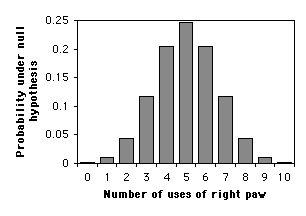
Let's say you want to know whether our cat, Gus, has a preference for one paw or uses both paws equally. You dangle a ribbon in his face and record which paw he uses to bat at it. You do this 10 times, and he bats at the ribbon with his right paw 8 times and his left paw 2 times. Then he gets bored with the experiment and leaves. Can you conclude that he is right-pawed, or could this result have occurred due to chance under the null hypothesis that he bats equally with each paw?

The null hypothesis is that each time Gus bats at the ribbon, the probability that he will use his right paw is 0.5. The probability that he will use his right paw on the first time is 0.5. The probability that he will use his right paw the first time AND the second time is 0.5 x 0.5, or 0.5², or 0.25. The probability that he will use his right paw all ten times is 0.5¹⁰, or about 0.001.

For a mixture of right and left paws, the calculation of the binomial distribution is more complicated. Where n is the total number of trials, k is the number of "successes" (statistical jargon for whichever event you want to consider), p is the expected proportion of successes if the null hypothesis is true, and Y is the probability of getting k successes in n trials, the equation is:

Y = pk(1-p)(n-k)n!
    ————————————
    k!(n-k)!

Fortunately, there's a spreadsheet function that does the calculation for you. To calculate the probability of getting exactly 8 out of 10 right paws, you would enter

=BINOMDIST(2, 10, 0.5, FALSE)

The first number, 2, is whichever event there are fewer than expected of; in this case, there are only two uses of the left paw, which is fewer than the expected 5. The second number, 10, is the total number of trials. The third number is the expected proportion of whichever event there were fewer than expected of, if the null hypothesis were true; here the null hypothesis predicts that half of all ribbon-battings will be with the left paw. And FALSE tells it to calculate the exact probability for that number of events only. In this case, the answer is P=0.044, so you might think it was significant at the P<0.05 level.

However, it would be incorrect to only calculate the probability of getting exactly 2 left paws and 8 right paws. Instead, you must calculate the probability of getting a deviation from the null expectation as large as, or larger than, the observed result. So you must calculate the probability that Gus used his left paw 2 times out of 10, or 1 time out of 10, or 0 times out of ten. Adding these probabilities together gives P=0.055, which is not quite significant at the P<0.05 level. You do this in a spreadsheet by entering

=BINOMDIST(2, 10, 0.5, TRUE).

The "TRUE" parameter tells the spreadsheet to calculate the sum of the probabilities of the observed number and all more extreme values; it's the equivalent of

=BINOMDIST(2, 10, 0.5, FALSE)+BINOMDIST(1, 10, 0.5, FALSE)+BINOMDIST(0, 10, 0.5, FALSE).

There's one more thing. The above calculation gives the total probability of getting 2, 1, or 0 uses of the left paw out of 10. However, the alternative hypothesis is that the number of uses of the right paw is not equal to the number of uses of the left paw. If there had been 2, 1, or 0 uses of the right paw, that also would have been an equally extreme deviation from the expectation. So you must add the probability of getting 2, 1, or 0 uses of the right paw, to account for both tails of the probability distribution; you are doing a two-tailed test. This gives you P=0.109, which is not very close to being significant. (If the null hypothesis had been 0.50 or more uses of the left paw, and the alternative hypothesis had been less than 0.5 uses of left paw, you could do a one-tailed test and use P=0.054. But you almost never have a situation where a one-tailed test is appropriate.)

The most common use of an exact binomial test is when the null hypothesis is that numbers of the two outcomes are equal. In that case, the meaning of a two-tailed test is clear, and you calculate the two-tailed P value by multiplying the one-tailed P value times two.

When the null hypothesis is not a 1:1 ratio, but something like a 3:1 ratio, statisticians disagree about the meaning of a two-tailed exact binomial test, and different statistical programs will give slightly different results. The simplest method is to use the binomial equation, as described above, to calculate the probability of whichever event is less common that expected, then multiply it by two. For example, let's say you've crossed a number of cats that are heterozygous at the hair-length gene; because short hair is dominant, you expect 75% of the kittens to have short hair and 25% to have long hair. You end up with 7 short haired and 5 long haired cats. There are 7 short haired cats when you expected 9, so you use the binomial equation to calculate the probability of 7 or fewer short-haired cats; this adds up to 0.158. Doubling this would give you a two-tailed P value of 0.315. This is what SAS and Richard Lowry's online calculator do.

The alternative approach is called the method of small P values, and I think most statisticians prefer it. For our example, you use the binomial equation to calculate the probability of obtaining exactly 7 out of 12 short-haired cats; it is 0.103. Then you calculate the probabilities for every other possible number of short-haired cats, and you add together those that are less than 0.103. That is the probabilities for 6, 5, 4 ... 0 short-haired cats, and in the other tail, only the probability of 12 out of 12 short-haired cats. Adding these probabilities gives a P value of 0.189. This is what my exact binomial spreadsheet does. I think the arguments in favor of the method of small P values make sense. If you are using the exact binomial test with expected proportions other than 50:50, make sure you specify which method you use (remember that it doesn't matter when the expected proportions are 50:50).

Sign test

One common application of the exact binomial test is known as the sign test. You use the sign test when there are two nominal variables and one measurement variable. One of the nominal variables has only two values, such as "before" and "after" or "left" and "right," and the other nominal variable identifies the pairs of observations. In a study of a hair-growth ointment, "amount of hair" would be the measurement variable, "before" and "after" would be the values of one nominal variable, and "Arnold," "Bob," "Charles" would be values of the second nominal variable.

The data for a sign test usually could be analyzed using a paired t–test or a Wilcoxon signed-rank test, if the null hypothesis is that the mean or median difference between pairs of observations is zero. However, sometimes you're not interested in the size of the difference, just the direction. In the hair-growth example, you might have decided that you didn't care how much hair the men grew or lost, you just wanted to know whether more than half of the men grew hair. In that case, you count the number of differences in one direction, count the number of differences in the opposite direction, and use the exact binomial test to see whether the numbers are different from a 1:1 ratio.

You should decide that a sign test is the test you want before you look at the data. If you analyze your data with a paired t–test and it's not significant, then you notice it would be significant with a sign test, it would be very unethical to just report the result of the sign test as if you'd planned that from the beginning.

Exact multinomial test

While the most common use of exact tests of goodness-of-fit is the exact binomial test, it is also possible to perform exact multinomial tests when there are more than two values of the nominal variable. The most common example in biology would be the results of genetic crosses, where one might expect a 1:2:1 ratio from a cross of two heterozygotes at one codominant locus, a 9:3:3:1 ratio from a cross of individuals heterozygous at two dominant loci, etc. The basic procedure is the same as for the exact binomial test: you calculate the probabilities of the observed result and all more extreme possible results and add them together. The underlying computations are more complicated, and if you have a lot of categories, your computer may have problems even if the total sample size is less than 1000. If you have a small sample size but so many categories that your computer program won't do an exact test, you can use a G–test or chi-square test of goodness-of-fit, but understand that the results may be somewhat inaccurate.

Post-hoc test

If you perform the exact multinomial test (with more than two categories) and get a significant result, you may want to follow up by testing whether each category deviates significantly from the expected number. It's a little odd to talk about just one category deviating significantly from expected; if there are more observations than expected in one category, there have to be fewer than expected in at least one other category. But looking at each category might help you understand better what's going on.

For example, let's say you do a genetic cross in which you expect a 9:3:3:1 ratio of purple, red, blue, and white flowers, and your observed numbers are 72 purple, 38 red, 20 blue, and 18 white. You do the exact test and get a P value of 0.0016, so you reject the null hypothesis. There are fewer purple and blue and more red and white than expected, but is there an individual color that deviates significantly from expected?

To answer this, do an exact binomial test for each category vs. the sum of all the other categories. For purple, compare the 72 purple and 76 non-purple to the expected 9:7 ratio. The P value is 0.07, so you can't say there are significantly fewer purple flowers than expected (although it's worth noting that it's close). There are 38 red and 110 non-red flowers; when compared to the expected 3:13 ratio, the P value is 0.035. This is below the significance level of 0.05, but because you're doing four tests at the same time, you need to correct for the multiple comparisons. Applying the Bonferroni correction, you divide the significance level (0.05) by the number of comparisons (4) and get a new significance level of 0.0125; since 0.035 is greater than this, you can't say there are significantly more red flowers than expected. Comparing the 18 white and 130 non-white to the expected ratio of 1:15, the P value is 0.006, so you can say that there are significantly more white flowers than expected.

It is possible that an overall significant P value could result from moderate-sized deviations in all of the categories, and none of the post-hoc tests will be significant. This would be frustrating; you'd know that something interesting was going on, but you couldn't say with statistical confidence exactly what it was.

I doubt that the procedure for post-hoc tests in a goodness-of-fit test that I've suggested here is original, but I can't find a reference to it; if you know who really invented this, e-mail me with a reference. And it seems likely that there's a better method that takes into account the non-independence of the numbers in the different categories (as the numbers in one category go up, the number in some other category must go down), but I have no idea what it might be.

Intrinsic hypothesis

You use exact test of goodness-of-fit that I've described here when testing fit to an extrinsic hypothesis, a hypothesis that you knew before you collected the data. For example, even before the kittens are born, you can predict that the ratio of short-haired to long-haired cats will be 3:1 in a genetic cross of two heterozygotes. Sometimes you want to test the fit to an intrinsic null hypothesis: one that is based on the data you collect, where you can't predict the results from the null hypothesis until after you collect the data. The only example I can think of in biology is Hardy-Weinberg proportions, where the number of each genotype in a sample from a wild population is expected to be p² or 2pq or q² (with more possibilities when there are more than two alleles); you don't know the allele frequencies (p and q) until after you collect the data. Exact tests of fit to Hardy-Weinberg raise a number of statistical issues and have received a lot of attention from population geneticists; if you need to do this, see Engels (2009) and the older references he cites. If you have biological data that you want to do an exact test of goodness-of-fit with an intrinsic hypothesis on, and it doesn't involve Hardy-Weinberg, e-mail me; I'd be very curious to see what kind of biological data requires this, and I will try to help you as best as I can.

Assumptions

Goodness-of-fit tests assume that the individual observations are independent, meaning that the value of one observation does not influence the value of other observations. To give an example, let's say you want to know what color flowers bees like. You plant four plots of flowers: one purple, one red, one blue, and one white. You get a bee, put it in a dark jar, carry it to a point equidistant from the four plots of flowers, and release it. You record which color flower it goes to first, then re-capture it and hold it prisoner until the experiment is done. You do this again and again for 100 bees. In this case, the observations are independent; the fact that bee #1 went to a blue flower has no influence on where bee #2 goes. This is a good experiment; if significantly more than 1/4 of the bees go to the blue flowers, it would be good evidence that the bees prefer blue flowers.

Now let's say that you put a beehive at the point equidistant from the four plots of flowers, and you record where the first 100 bees go. If the first bee happens to go to the plot of blue flowers, it will go back to the hive and do its bee-butt-wiggling dance that tells the other bees, "Go 15 meters southwest, there's a bunch of yummy nectar there!" Then some more bees will fly to the blue flowers, and when they return to the hive, they'll do the same bee-butt-wiggling dance. The observations are NOT independent; where bee #2 goes is strongly influenced by where bee #1 happened to go. If "significantly" more than 1/4 of the bees go to the blue flowers, it could easily be that the first bee just happened to go there by chance, and bees may not really care about flower color.

Examples

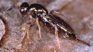
Roptrocerus xylophagorum is a parasitoid of bark beetles. To determine what cues these wasps use to find the beetles, Sullivan et al. (2000) placed female wasps in the base of a Y-shaped tube, with a different odor in each arm of the Y, then counted the number of wasps that entered each arm of the tube. In one experiment, one arm of the Y had the odor of bark being eaten by adult beetles, while the other arm of the Y had bark being eaten by larval beetles. Ten wasps entered the area with the adult beetles, while 17 entered the area with the larval beetles. The difference from the expected 1:1 ratio is not significant (P=0.248). In another experiment that compared infested bark with a mixture of infested and uninfested bark, 36 wasps moved towards the infested bark, while only 7 moved towards the mixture; this is significantly different from the expected ratio (P=9×10^-6).

---

Yukilevich and True (2008) mixed 30 male and 30 female Drosophila melanogaster from Alabama with 30 male and 30 females from Grand Bahama Island. They observed 246 matings; 140 were homotypic (male and female from the same location), while 106 were heterotypic (male and female from different locations). The null hypothesis is that the flies mate at random, so that there should be equal numbers of homotypic and heterotypic matings. There were significantly more homotypic matings (exact binomial test, P=0.035) than heterotypic.

---

As an example of the sign test, Farrell et al. (2001) estimated the evolutionary tree of two subfamilies of beetles that burrow inside trees as adults. They found ten pairs of sister groups in which one group of related species, or "clade," fed on angiosperms and one fed on gymnosperms, and they counted the number of species in each clade. There are two nominal variables, food source (angiosperms or gymnosperms) and pair of clades (Corthylina vs. Pityophthorus, etc.) and one measurement variable, the number of species per clade.

The biological null hypothesis is that although the number of species per clade may vary widely due to a variety of unknown factors, whether a clade feeds on angiosperms or gymnosperms will not be one of these factors. In other words, you expect that each pair of related clades will differ in number of species, but half the time the angiosperm-feeding clade will have more species, and half the time the gymnosperm-feeding clade will have more species.

Applying a sign test, there are 10 pairs of clades in which the angiosperm-specialized clade has more species, and 0 pairs with more species in the gymnosperm-specialized clade; this is significantly different from the null expectation (P=0.002), and you can reject the null hypothesis and conclude that in these beetles, clades that feed on angiosperms tend to have more species than clades that feed on gymnosperms.

Angiosperm-feeding	Spp.		Gymonsperm-feeding	Spp.
Corthylina	458		Pityophthorus	200
Scolytinae	5200		Hylastini+Tomacini	180
Acanthotomicus+Premnobious	123		Orhotomicus	11
Xyleborini/Dryocoetini	1500		Ipini	195
Apion	1500		Antliarhininae	12
Belinae	150		Allocoryninae+Oxycorinae	30
Higher Curculionidae	44002		Nemonychidae	85
Higher Cerambycidae	25000		Aseminae + Spondylinae	78
Megalopodinae	400		Palophaginae	3
Higher Chrysomelidae	33400		Aulocoscelinae + Orsodacninae	26

---

Mendel (1865) crossed pea plants that were heterozygotes for green pod/yellow pod; pod color is the nominal variable, with "green" and "yellow" as the values. If this is inherited as a simple Mendelian trait, with green dominant over yellow, the expected ratio in the offspring is 3 green: 1 yellow. He observed 428 green and 152 yellow. The expected numbers of plants under the null hypothesis are 435 green and 145 yellow, so Mendel observed slightly fewer green-pod plants than expected. The P value for an exact binomial test using the method of small P values, as implemented in my spreadsheet, is 0.533, indicating that the null hypothesis cannot be rejected; there is no significant difference between the observed and expected frequencies of pea plants with green pods. (SAS uses a different method that gives a P value of 0.530. With a smaller sample size, the difference between the "method of small P values" that I and most statisticians prefer, and the cruder method that SAS uses, could be large enough to be important.)

---

Mendel (1865) also crossed peas that were heterozygous at two genes: one for yellow vs. green, the other for round vs. wrinkled; yellow was dominant over green, and round was dominant over wrinkled. The expected and observed results were:

phenotype	expected proportion	expected number	observed number
yellow+round	9	312.75	315
green+round	3	104.25	108
yellow+wrinkled	3	104.25	101
round+wrinkled	1	34.75	32

This is an example of the exact multinomial test, since there are four categories, not two. The P value is 0.93, so the difference between observed and expected is nowhere near significance.

Graphing the results

You plot the results of an exact test the same way would any other goodness-of-fit test.

Similar tests

A G–test or chi-square goodness-of-fit test could also be used for the same data as the exact test of goodness-of-fit. Where the expected numbers are small, the exact test will give more accurate results than the G–test or chi-squared tests. Where the sample size is large (over a thousand), attempting to use the exact test may give error messages (computers have a hard time calculating factorials for large numbers), so a G–test or chi-square test must be used. For intermediate sample sizes, all three tests give approximately the same results. I recommend that you use the exact test when n is less than 1000; see the web page on small sample sizes for further discussion.

If you try to do an exact test with a large number of categories, your computer may not be able to do the calculations even if your total sample size is less than 1000. In that case, you can cautiously use the G–test or chi-square goodness-of-fit test, knowing that the results may be somewhat inaccurate.

The exact test of goodness-of-fit is not the same as Fisher's exact test of independence. You use a test of independence for two nominal variables, such as sex and location. If you wanted to compare the ratio of males to female students at Delaware to the male:female ratio at Maryland, you would use a test of independence; if you want to compare the male:female ratio at Delaware to a theoretical 1:1 ratio, you would use a goodness-of-fit test.

How to do the test

Spreadsheet

I have set up a spreadsheet that performs the exact binomial test for sample sizes up to 1000. It is self-explanatory. It uses the method of small P values when the expected proportions are different from 50:50.

Web page

Richard Lowry has set up a web page that does the exact binomial test. It does not use the method of small P values, so I do not recommend it if your expected proportions are different from 50:50. I'm not aware of any web pages that will do the exact binomial test using the method of small P values, and I'm not aware of any web pages that will do exact multinomial tests.

R

Salvatore Mangiafico's R Companion has a sample R program for the exact test of goodness-of-fit.

SAS

Here is a sample SAS program, showing how to do the exact binomial test on the Gus data. The "P=0.5" gives the expected proportion of whichever value of the nominal variable is alphabetically first; in this case, it gives the expected proportion of "left."

The SAS exact binomial function finds the two-tailed P value by doubling the P value of one tail. The binomial distribution is not symmetrical when the expected proportion is other than 50%%, so the technique SAS uses isn't as good as the method of small P values. I don't recommend doing the exact binomial test in SAS when the expected proportion is anything other than 50%.

DATA gus;
   INPUT paw $;
   DATALINES;
right
left
right
right
right
right
left
right
right
right
;
PROC FREQ DATA=gus;
   TABLES paw / BINOMIAL(P=0.5);
   EXACT BINOMIAL;
RUN;

Near the end of the output is this:

Exact Test                         
One-sided Pr <=  P           0.0547
Two-sided = 2 * One-sided    0.1094

The "Two-sided=2*One-sided" number is the two-tailed P value that you want.

If you have the total numbers, rather than the raw values, you'd use a WEIGHT parameter in PROC FREQ. The ZEROS option tells it to include observations with counts of zero, for example if Gus had used his left paw 0 times; it doesn't hurt to always include the ZEROS option.

DATA gus;
   INPUT paw $ count;
   DATALINES;
right 10
left 2
;
PROC FREQ DATA=gus;
   WEIGHT count / ZEROS; 
   TABLES paw / BINOMIAL(P=0.5);
EXACT BINOMIAL;
RUN;

This example shows how do to the exact multinomial test. The numbers are Mendel's data from a genetic cross in which you expect a 9:3:3:1 ratio of peas that are round+yellow, round+green, wrinkled+yellow, and wrinkled+green. The ORDER=DATA option tells SAS to analyze the data in the order they are input (rndyel, rndgrn, wrnkyel, wrnkgrn, in this case), not alphabetical order. The TESTP=(0.5625 0.1875 0.0625 0.1875) lists the expected proportions in the same order.

DATA peas;
   INPUT color $ count;
   DATALINES;
rndyel 315
rndgrn 108
wrnkyel 101
wrnkgrn 32
;
PROC FREQ DATA=peas ORDER=DATA;
   WEIGHT count / ZEROS;
   TABLES color / CHISQ TESTP=(0.5625 0.1875 0.1875 0.0625);
   EXACT CHISQ;
RUN;

The P value you want is labeled "Exact Pr >= ChiSq":

     Chi-Square Test
for Specified Proportions
-------------------------------------
Chi-Square                     0.4700
DF                                  3
Asymptotic Pr >  ChiSq         0.9254
Exact      Pr >= ChiSq         0.9272

Power analysis

Before you do an experiment, you should do a power analysis to estimate the sample size you'll need. To do this for an exact binomial test using G*Power, choose "Exact" under "Test Family" and choose "Proportion: Difference from constant" under "Statistical test." Under "Type of power analysis", choose "A priori: Compute required sample size". For "Input parameters," enter the number of tails (you'll almost always want two), alpha (usually 0.05), and Power (often 0.5, 0.8, or 0.9). The "Effect size" is the difference in proportions between observed and expected that you hope to see, and the "Constant proportion" is the expected proportion for one of the two categories (whichever is smaller). Hit "Calculate" and you'll get the Total Sample Size.

As an example, let's say you wanted to do an experiment to see if Gus the cat really did use one paw more than the other for getting my attention. The null hypothesis is that the probability that he uses his left paw is 0.50, so enter that in "Constant proportion". You decide that if the probability of him using his left paw is 0.40, you want your experiment to have an 80% probability of getting a significant (P<0.05) result, so enter 0.10 for Effect Size, 0.05 for Alpha, and 0.80 for Power. If he uses his left paw 60% of the time, you'll accept that as a significant result too, so it's a two-tailed test. The result is 199. This means that if Gus really is using his left paw 40% (or 60%) of the time, a sample size of 199 observations will have an 80% probability of giving you a significant (P<0.05) exact binomial test.

Many power calculations for the exact binomial test, like G*Power, find the smallest sample size that will give the desired power, but there is a "sawtooth effect" in which increasing the sample size can actually reduce the power. Chernick and Liu (2002) suggest finding the smallest sample size that will give the desired power, even if the sample size is increased. For the Gus example, the method of Chernick and Liu gives a sample size of 210, rather than the 199 given by G*Power. Because both power and effect size are usually just arbitrary round numbers, where it would be easy to justify other values that would change the required sample size, the small differences in the method used to calculate desired sample size are probably not very important. The only reason I mention this is so that you won't be alarmed if different power analysis programs for the exact binomial test give slightly different results for the same parameters.

G*Power does not do a power analysis for the exact test with more than two categories. If you have to do a power analysis and your nominal variable has more than two values, use the power analysis for chi-square tests in G*Power instead. The results will be pretty close to a true power analysis for the exact multinomial test, and given the arbitrariness of parameters like power and effect size, the results should be close enough.

References

Picture of wasp from Universal Chalcidoidea Database.

Chernick, M.R., and C.Y. Liu. 2002. The saw-toothed behavior of power versus sample size and software solutions: single binomial proportion using exact methods. American Statistician 56: 149-155.

Engels, W.R. 2009. Exact tests for Hardy-Weinberg proportions. Genetics 183: 1431-1441.

Farrell, B.D., A.S. Sequeira, B.C. O'Meara, B.B. Normark, J.H. Chung, and B.H. Jordal. 2001. The evolution of agriculture in beetles (Curculionidae: Scolytinae and Platypodinae). Evolution 55: 2011-2027.

Mendel, G. 1865. Experiments in plant hybridization. available at MendelWeb.

Sullivan, B.T., E.M. Pettersson, K.C. Seltmann, and C.W. Berisford. 2000. Attraction of the bark beetle parasitoid Roptrocerus xylophagorum (Hymenoptera: Pteromalidae) to host-associated olfactory cues. Environmental Entomology 29: 1138-1151.

Yukilevich, R., and J.R. True. 2008. Incipient sexual isolation among cosmopolitan Drosophila melanogaster populations. Evolution 62: 2112-2121.

---

⇐ Previous topic|Next topic ⇒
Table of Contents

---

This page was last revised July 20, 2015. Its address is http://www.biostathandbook.com/exactgof.html. It may be cited as:
McDonald, J.H. 2014. Handbook of Biological Statistics (3rd ed.). Sparky House Publishing, Baltimore, Maryland. This web page contains the content of pages 29-39 in the printed version.

©2014 by John H. McDonald. You can probably do what you want with this content; see the permissions page for details.