
⇐ Previous topic|Next topic ⇒
Table of Contents
Fisher's exact test of independence
Summary
Use the Fisher's exact test of independence when you have two nominal variables and you want to see whether the proportions of one variable are different depending on the value of the other variable. Use it when the sample size is small.
When to use it
Use Fisher's exact test when you have two nominal variables. You want to know whether the proportions for one variable are different among values of the other variable. For example, van Nood et al. (2013) studied patients with Clostridium difficile infections, which cause persistent diarrhea. One nominal variable was the treatment: some patients were given the antibiotic vancomycin, and some patients were given a fecal transplant. The other nominal variable was outcome: each patient was either cured or not cured. The percentage of people who received one fecal transplant and were cured (13 out of 16, or 81%) is higher than the percentage of people who received vancomycin and were cured (4 out of 13, or 31%), which seems promising, but the sample sizes seem kind of small. Fisher's exact test will tell you whether this difference between 81 and 31% is statistically significant.
A data set like this is often called an "R×C table," where R is the number of rows and C is the number of columns. The fecal-transplant vs. vancomycin data I'm using as an example is a 2×2 table. van Nood et al. (2013) actually had a third treatment, 13 people given vancomycin plus a bowel lavage, making the total data set a 2×3 table (or a 3×2 table; it doesn't matter which variable you call the rows and which the columns). The most common use of Fisher's exact test is for 2×2 tables, so that's mostly what I'll describe here.
Fisher's exact test is more accurate than the chi-square test or G–test of independence when the expected numbers are small. I recommend you use Fisher's exact test when the total sample size is less than 1000, and use the chi-square or G–test for larger sample sizes. See the web page on small sample sizes for further discussion of what it means to be "small".
Null hypothesis
The null hypothesis is that the relative proportions of one variable are independent of the second variable; in other words, the proportions at one variable are the same for different values of the second variable. In the C. difficile example, the null hypothesis is that the probability of getting cured is the same whether you receive a fecal transplant or vancomycin.
How the test works
Unlike most statistical tests, Fisher's exact test does not use a mathematical function that estimates the probability of a value of a test statistic; instead, you calculate the probability of getting the observed data, and all data sets with more extreme deviations, under the null hypothesis that the proportions are the same. For the C. difficile experiment, there are 3 sick and 13 cured fecal-transplant patients, and 9 sick and 4 cured vancomycin patients. Given that there are 16 total fecal-transplant patients, 13 total vancomycin patients, and 12 total sick patients, you can use the "hypergeometric distribution" (please don't ask me to explain it) to calculate the probability of getting these numbers:
| fecal | vancomycin | |
|---|---|---|
| sick | 3 | 9 |
| cured | 13 | 4 |
Next you calculate the probability of more extreme ways of distributing the 12 sick people:
| fecal | vancomycin | |
|---|---|---|
| sick | 2 | 10 |
| cured | 14 | 3 |
| fecal | vancomycin | |
|---|---|---|
| sick | 1 | 11 |
| cured | 15 | 2 |
| fecal | vancomycin | |
|---|---|---|
| sick | 0 | 12 |
| cured | 16 | 1 |
To calculate the probability of 3, 2, 1, or 0 sick people in the fecal-transplant group, you add the four probabilities together to get P=0.00840. This is the one-tailed P value, which is hardly ever what you want. In our example experiment, you would use a one-tailed test only if you decided, before doing the experiment, that you were only interested in a result that had fecal transplants being better than vancomycin, not if fecal transplants were worse; in other words, you decided ahead of time that your null hypothesis was that the proportion of sick fecal transplant people was the same as, or greater than, sick vancomycin people. Ruxton and Neuhauser (2010) surveyed articles in the journal Behavioral Ecology and Sociobiology and found several that reported the results of one-tailed Fisher's exact tests, even though two-tailed would have been more appropriate. Apparently some statistics textbooks and programs perpetuate confusion about one-tailed vs. two-tailed Fisher's tests. You should almost always use a two-tailed test, unless you have a very good reason.
For the usual two-tailed test, you also calculate the probability of getting deviations as extreme as the observed, but in the opposite direction. This raises the issue of how to measure "extremeness." There are several different techniques, but the most common is to add together the probabilities of all combinations that have lower probabilities than that of the observed data. Martín Andrés and Herranz Tejedor (1995) did some computer simulations that show that this is the best technique, and it's the technique used by SAS and most of the web pages I've seen. For our fecal example, the extreme deviations in the opposite direction are those with P<0.00772, which are the tables with 0 or 1 sick vancomycin people. These tables have P=0.000035 and P=0.00109, respectively. Adding these to the one-tailed P value (P=0.00840) gives you the two-tailed P value, P=0.00953.
Post-hoc tests
When analyzing a table with more than two rows or columns, a significant result will tell you that there is something interesting going on, but you will probably want to test the data in more detail. For example, Fredericks (2012) wanted to know whether checking termite monitoring stations frequently would scare termites away and make it harder to detect termites. He checked the stations (small bits of wood in plastic tubes, placed in the ground near termite colonies) either every day, every week, every month, or just once at the end of the three-month study, and recorded how many had termite damage by the end of the study:
| Termite damage | No termites | Percent termite damage | |
|---|---|---|---|
| Daily | 1 | 24 | 4% |
| Weekly | 5 | 20 | 20% |
| Monthly | 14 | 11 | 56% |
| Quarterly | 11 | 14 | 44% |
The overall P value for this is P=0.00012, so it is highly significant; the frequency of disturbance is affecting the presence of termites. That's nice to know, but you'd probably want to ask additional questions, such as whether the difference between daily and weekly was significant, or the difference between weekly and monthly. You could do a 2×2 Fisher's exact test for each of these pairwise comparisons, but there are 6 possible pairs, so you need to correct for the multiple comparisons. One way to do this is with a modification of the Bonferroni-corrected pairwise technique suggested by MacDonald and Gardner (2000), substituting Fisher's exact test for the chi-square test they used. You do a Fisher's exact test on each of the 6 possible pairwise comparisons (daily vs. weekly, daily vs. monthly, etc.), then apply the Bonferroni correction for multiple tests. With 6 pairwise comparisons, the P value must be less than 0.05/6, or 0.008, to be significant at the P<0.05 level. Two comparisons (daily vs. monthly and daily vs. quarterly) are therefore significant
| P value | |
|---|---|
| Daily vs. weekly | 0.189 |
| Daily vs. monthly | 0.00010 |
| Daily vs. quarterly | 0.0019 |
| Weekly vs. monthly | 0.019 |
| Weekly vs. quarterly | 0.128 |
| Monthly vs. quarterly | 0.57 |
You could have decided, before doing the experiment, that testing all possible pairs would make it too hard to find a significant difference, so instead you would just test each treatment vs. quarterly. This would mean there were only 3 possible pairs, so each pairwise P value would have to be less than 0.05/3, or 0.017, to be significant. That would give you more power, but it would also mean that you couldn't change your mind after you saw the data and decide to compare daily vs. monthly.
Assumptions
Independence
Fisher's exact test, like other tests of independence, assumes that the individual observations are independent.
Fixed totals
Unlike other tests of independence, Fisher's exact test assumes that the row and column totals are fixed, or "conditioned." An example would be putting 12 female hermit crabs and 9 male hermit crabs in an aquarium with 7 red snail shells and 14 blue snail shells, then counting how many crabs of each sex chose each color (you know that each hermit crab will pick one shell to live in). The total number of female crabs is fixed at 12, the total number of male crabs is fixed at 9, the total number of red shells is fixed at 7, and the total number of blue shells is fixed at 14. You know, before doing the experiment, what these totals will be; the only thing you don't know is how many of each sex-color combination there are.
There are very few biological experiments where both the row and column totals are conditioned. In the much more common design, one or two of the row or column totals are free to vary, or "unconditioned." For example, in our C. difficile experiment above, the numbers of people given each treatment are fixed (16 given a fecal transplant, 13 given vancomycin), but the total number of people who are cured could have been anything from 0 to 29. In the moray eel experiment below, both the total number of each species of eel, and the total number of eels in each habitat, are unconditioned.
When one or both of the row or column totals are unconditioned, the Fisher's exact test is not, strictly speaking, exact. Instead, it is somewhat conservative, meaning that if the null hypothesis is true, you will get a significant (P<0.05) P value less than 5% of the time. This makes it a little less powerful (harder to detect a real difference from the null, when there is one). Statisticians continue to argue about alternatives to Fisher's exact test, but the improvements seem pretty small for reasonable sample sizes, with the considerable cost of explaining to your readers why you are using an obscure statistical test instead of the familiar Fisher's exact test. I think most biologists, if they saw you get a significant result using Barnard's test, or Boschloo's test, or Santner and Snell's test, or Suissa and Shuster's test, or any of the many other alternatives, would quickly run your numbers through Fisher's exact test. If your data weren't significant with Fisher's but were significant with your fancy alternative test, they would suspect that you fished around until you found a test that gave you the result you wanted, which would be highly evil. Even though you may have really decided on the obscure test ahead of time, you don't want cynical people to think you're evil, so stick with Fisher's exact test.
Examples

The eastern chipmunk trills when pursued by a predator, possibly to warn other chipmunks. Burke da Silva et al. (2002) released chipmunks either 10 or 100 meters from their home burrow, then chased them (to simulate predator pursuit). Out of 24 female chipmunks released 10 m from their burrow, 16 trilled and 8 did not trill. When released 100 m from their burrow, only 3 female chipmunks trilled, while 18 did not trill. The two nominal variables are thus distance from the home burrow (because there are only two values, distance is a nominal variable in this experiment) and trill vs. no trill. Applying Fisher's exact test, the proportion of chipmunks trilling is significantly higher (P=0.0007) when they are closer to their burrow.
McDonald and Kreitman (1991) sequenced the alcohol dehydrogenase gene in several individuals of three species of Drosophila. Varying sites were classified as synonymous (the nucleotide variation does not change an amino acid) or amino acid replacements, and they were also classified as polymorphic (varying within a species) or fixed differences between species. The two nominal variables are thus substitution type (synonymous or replacement) and variation type (polymorphic or fixed). In the absence of natural selection, the ratio of synonymous to replacement sites should be the same for polymorphisms and fixed differences. There were 43 synonymous polymorphisms, 2 replacement polymorphisms, 17 synonymous fixed differences, and 7 replacement fixed differences.
| Synonymous | Replacement | |
|---|---|---|
| polymorphisms | 43 | 2 |
| fixed | 17 | 7 |
The result is P=0.0067, indicating that the null hypothesis can be rejected; there is a significant difference in synonymous/replacement ratio between polymorphisms and fixed differences. (Note that we used a G–test of independence in the original McDonald and Kreitman [1991] paper, which is a little embarrassing in retrospect, since I'm now telling you to use Fisher's exact test for such small sample sizes; fortunately, the P value we got then, P=0.006, is almost the same as with the more appropriate Fisher's test.)
Descamps et al. (2009) tagged 50 king penguins (Aptenodytes patagonicus) in each of three nesting areas (lower, middle, and upper) on Possession Island in the Crozet Archipelago, then counted the number that were still alive a year later, with these results:
| Alive | Dead | |
|---|---|---|
| Lower nesting area | 43 | 7 |
| Middle nesting area | 44 | 6 |
| Upper nesting area | 49 | 1 |
Seven penguins had died in the lower area, six had died in the middle area, and only one had died in the upper area. Descamps et al. analyzed the data with a G–test of independence, yielding a significant (P=0.048) difference in survival among the areas; however, analyzing the data with Fisher's exact test yields a non-significant (P=0.090) result.
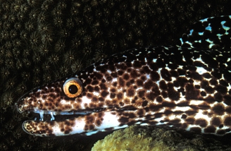
Young and Winn (2003) counted sightings of the spotted moray eel, Gymnothorax moringa, and the purplemouth moray eel, G. vicinus, in a 150-m by 250-m area of reef in Belize. They identified each eel they saw, and classified the locations of the sightings into three types: those in grass beds, those in sand and rubble, and those within one meter of the border between grass and sand/rubble. The number of sightings are shown in the table, with percentages in parentheses:
| G. moringa | G. vicinus | Percent G. vicinus |
|
|---|---|---|---|
| Grass | 127 | 116 | 47.7% |
| Sand | 99 | 67 | 40.4% |
| Border | 264 | 161 | 37.9% |
The nominal variables are the species of eel (G. moringa or G. vicinus) and the habitat type (grass, sand, or border). The difference in habitat use between the species is significant (P=0.044).
Custer and Galli (2002) flew a light plane to follow great blue herons (Ardea herodias) and great egrets (Casmerodius albus) from their resting site to their first feeding site at Peltier Lake, Minnesota, and recorded the type of substrate each bird landed on.
| Heron | Egret | |
|---|---|---|
| Vegetation | 15 | 8 |
| Shoreline | 20 | 5 |
| Water | 14 | 7 |
| Structures | 6 | 1 |
Fisher's exact test yields P=0.54, so there is no evidence that the two species of birds use the substrates in different proportions.
Graphing the results
You plot the results of Fisher's exact test the same way would any other test of independence.
Similar tests
You can use the chi-square test of independence or the G–test of independence on the same kind of data as Fisher's exact test. When some of the expected values are small, Fisher's exact test is more accurate than the chi-square or G–test of independence. If all of the expected values are very large, Fisher's exact test becomes computationally impractical; fortunately, the chi-square or G–test will then give an accurate result. The usual rule of thumb is that Fisher's exact test is only necessary when one or more expected values are less than 5, but this is a remnant of the days when doing the calculations for Fisher's exact test was really hard. I recommend using Fisher's exact test for any experiment with a total sample size less than 1000. See the web page on small sample sizes for further discussion of the boundary between "small" and "large."
You should use McNemar's test when the two samples are not independent, but instead are two sets of pairs of observations. Often, each pair of observations is made on a single individual, such as individuals before and after a treatment or individuals diagnosed using two different techniques. For example, Dias et al. (2014) surveyed 62 men who were circumcised as adults. Before circumcision, 6 of the 62 men had erectile dysfunction; after circumcision, 16 men had erectile dysfunction. This may look like data suitable for Fisher's exact test (two nominal variables, erect vs. flaccid and before vs. after circumcision), and if analyzed that way, the result would be P=0.033. However, we know more than just how many men had erectile dysfunction, we know that 10 men switched from normal function to dysfunction after circumcision, and 0 men switched from dysfunction to normal. The statistical null hypothesis of McNemar's test is that the number of switchers in one direction is equal to the number of switchers in the opposite direction. McNemar's test compares the observed data to the null expectation using a goodness-of-fit test. The numbers are almost always small enough that you can make this comparison using the exact test of goodness-of-fit. For the example data of 10 switchers in one direction and 0 in the other direction, McNemar's test gives P=0.002; this is a much smaller P value than the result from Fisher's exact test. McNemar's test doesn't always give a smaller P value than Fisher's. If all 6 men in the Dias et al. (2014) study with erectile dysfunction before circumcision had switched to normal function, and 16 men had switched from normal function before circumcision to erectile dysfunction, the P value from McNemar's test would have been 0.052.
How to do the test
Spreadsheet
I've written a spreadsheet to perform Fisher's exact test for 2×2 tables. It handles samples with the smaller column total less than 500.
Web pages
Several people have created web pages that perform Fisher's exact test for 2×2 tables. I like Øyvind Langsrud's web page for Fisher's exact test. Just enter the numbers into the cells on the web page, hit the Compute button, and get your answer. You should almost always use the "2-tail P value" given by the web page.
There is also a web page for Fisher's exact test for up to 6×6 tables. It will only take data with fewer than 100 observations in each cell.
R
Salvatore Mangiafico's R Companion has a sample R program for Fisher's exact test and another for McNemar's test.
SAS
Here is a SAS program that uses PROC FREQ for a Fisher's exact test. It uses the chipmunk data from above.
DATA chipmunk;
   INPUT distance $ sound $ count;
   DATALINES;
10m  trill   16
10m  notrill  8
100m trill    3
100m notrill 18
;
PROC FREQ DATA=chipmunk;
   WEIGHT count / ZEROS;
   TABLES distance*sound / FISHER;
RUN;
The output includes the following:
       Fisher's Exact Test
----------------------------------
Cell (1,1) Frequency (F)        18
Left-sided Pr <= F          1.0000
Right-sided Pr >= F      4.321E-04

Table Probability (P)       4.012E-04
Two-sided Pr <= P        6.862E-04
The "Two-sided Pr <= P" is the two-tailed P value that you want.
The output looks a little different when you have more than two rows or columns. Here is an example using the data on heron and egret substrate use from above:
DATA birds;
   INPUT bird $ substrate $ count;
   DATALINES;
heron vegetation 15
heron shoreline  20
heron water      14
heron structures  6
egret vegetation  8
egret shoreline   5
egret water       7
egret structures  1
;
PROC FREQ DATA=birds;
   WEIGHT count / ZEROS;
   TABLES bird*substrate / FISHER;
RUN;
The results of the exact test are labeled "Pr <= P"; in this case, P=0.5491.
       Fisher's Exact Test
----------------------------------
Table Probability (P)       0.0073
Pr <= P                     0.5491
Power analysis
The G*Power program will calculate the sample size needed for a 2×2 test of independence, whether the sample size ends up being small enough for a Fisher's exact test or so large that you must use a chi-square or G–test. Choose "Exact" from the "Test family" menu and "Proportions: Inequality, two independent groups (Fisher's exact test)" from the "Statistical test" menu. Enter the proportions you hope to see, your alpha (usually 0.05) and your power (usually 0.80 or 0.90). If you plan to have more observations in one group than in the other, you can make the "Allocation ratio" different from 1.
As an example, let's say you're looking for a relationship between bladder cancer and genotypes at a polymorphism in the catechol-O-methyltransferase gene in humans. Based on previous research, you're going to pool together the GG and GA genotypes and compare these "GG+GA" and AA genotypes. In the population you're studying, you know that the genotype frequencies in people without bladder cancer are 0.84 GG+GA and 0.16 AA; you want to know how many people with bladder cancer you'll have to genotype to get a significant result if they have 6% more AA genotypes. It's easier to find controls than people with bladder cancer, so you're planning to have twice as many people without bladder cancer. On the G*Power page, enter 0.16 for proportion p1, 0.22 for proportion p2, 0.05 for alpha, 0.80 for power, and 0.5 for allocation ratio. The result is a total sample size of 1523, so you'll need 508 people with bladder cancer and 1016 people without bladder cancer.
Note that the sample size will be different if your effect size is a 6% lower frequency of AA in bladder cancer patients, instead of 6% higher. If you don't have a strong idea about which direction of difference you're going to see, you should do the power analysis both ways and use the larger sample size estimate.
If you have more than two rows or columns, use the power analysis for chi-square tests of independence. The results should be close enough to correct, even if the sample size ends up being small enough for Fisher's exact test.
References
Burke da Silva, K., C. Mahan, and J. da Silva. 2002. The trill of the chase: eastern chipmunks call to warn kin. Journal of Mammalogy 83: 546-552.
Custer, C.M., and J. Galli. 2002. Feeding habitat selection by great blue herons and great egrets nesting in east central Minnesota. Waterbirds 25: 115-124.
Descamps, S., C. le Bohec, Y. le Maho, J.-P. Gendner, and M. Gauthier-Clerc. 2009. Relating demographic performance to breeding-site location in the king penguin. Condor 111: 81-87.
Dias, J., R. Freitas, R. Amorim, P. Espiridião, L. Xambre and L. Ferraz. 2014. Adult circumcision and male sexual health: a retrospective analysis. Andrologia 46: 459-464.
Fredericks, J.G. 2012. Factors influencing foraging behavior and bait station discovery by subterranean termites (Reticulitermes spp.) (Blattodea: Rhinotermitidae) in Lewes, Delaware. Ph.D. dissertation, University of Delaware.
MacDonald, P.L., and Gardner, R.C. 2000. Type I error rate comparisons of post hoc procedures for I×J chi-square tables. Educational and Psychological Measurment 60: 735-754.
Martín Andrés, A, and I. Herranz Tejedor. 1995. Is Fisher's exact test very conservative? Computational Statistics and Data Analysis 19: 579–591.
McDonald, J.H. and M. Kreitman. 1991. Adaptive protein evolution at the Adh locus in Drosophila. Nature 351: 652-654.
Ruxton, G.D., and M. Neuhäuser. 2010. Good practice in testing for an association in contingency tables. Behavioral Ecology and Sociobiology 64: 1501-1513.
van Nood, E., Vrieze, A., Nieuwdorp, M., et al. (13 co-authors). 2013. Duodenal infusion of donor feces for recurrent Clostridium difficile. New England Journal of Medicine 368: 407-415.
Young, R.F., and H.E. Winn. 2003. Activity patterns, diet, and shelter site use for two species of moray eels, Gymnothorax moringa and Gymnothorax vicinus, in Belize. Copeia 2003: 44-55.
⇐ Previous topic|Next topic ⇒
Table of Contents
This page was last revised July 20, 2015. Its address is http://www.biostathandbook.com/fishers.html. It may be cited as:
McDonald, J.H. 2014. Handbook of Biological Statistics (3rd ed.). Sparky House Publishing, Baltimore, Maryland. This web page contains the content of pages 77-85 in the printed version.
©2014 by John H. McDonald. You can probably do what you want with this content; see the permissions page for details.